The latest update of ArcGIS Business Analyst Web App expands users’ analytical horizons by providing a new Results pane in the popular smart map search workflow. Smart map search allows you to view areas on the map that match criteria you define. For example, you might start with a question, such as “Which counties in the United States have a lower life expectancy than the current national average of 76.4 years?” This is the type of question for which smart map search can provide a straightforward visualization and answer.

But what if you haven’t yet formulated your question? Let’s say you’ve found a great dataset, such as the County Health Rankings data compiled by the University of Wisconsin Population Health Institute. You want to explore this data on the map, but don’t know yet precisely which ranges and filters to apply. The Results pane can assist you in performing a sophisticated data exploration to learn more about the data and what questions you might use it to answer.
Data exploration in smart map search
Exploratory data analysis (EDA) is an essential step in understanding datasets. Through EDA, you can uncover patterns within the data, summarize its key features, detect outliers, test a hypothesis, and reveal relationships among the variables.
In this blog article, we’ll demonstrate how to use the smart map search Results pane in Business Analyst Web App for exploratory data analysis, using 2023 County Health Rankings data as our example. Specifically, we’ll focus on examining average life expectancy across various race groups. We will also analyze the extent to which variations in life expectancy can be attributed to median household income and food insecurity. By following the steps detailed below, you’ll be well-equipped to conduct your own exploratory data analysis, and also gain a deeper understanding of the factors that influence life expectancy in the United States.
Step 1: Gain a comprehensive overview
The starting point for any exploratory data analysis is to take a broad overview of the dataset. Using County Health Rankings (CHR) data, we’ll collect average life expectancy statistics for each group at the county level, providing a quick overview of general trends in life expectancy across different demographic groups in the U.S. This first step offers a comprehensive insight into the differences among race groups.
After opening Business Analyst and creating a project, we follow these steps to add CHR data to our project:
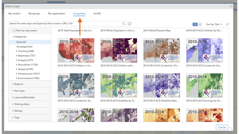
- Click Add data and click Web maps and layers.
- Click the Living Atlas tab and search for “County Health Rankings 2023” and click the map to open it.

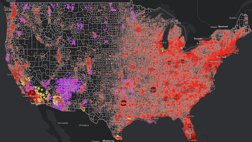
The map now displays the CHR map, and its data is now saved to our project. The map is color-coded by county, using a dark purple-to-light yellow color ramp. Each county’s color corresponds to the percentage of adults in that county that report fair or poor health. It’s an immediately legible and compelling visualization—but did you know that the CHR data actually contains more than the web map? There are tons of health-related variables as well!
To begin exploratory data analysis, we’ll open the smart map search workflow:
- Click Create maps and choose Smart map search.

By default, the map currently displays the Percentage of adults that report fair or poor health variable. We will look through the other variables in the dataset, and configure it to show average life expectancy variables:
- At the bottom of the workflow pane, click Browse all variables.
- On the Standard data tab, choose Map layers.
- Expand the County (Map Layers) section and find this variable: Average expected number of years from birth. Select the check box for this variable for the five race groups.
- Find and add the Median household income and Percentage of population who are food insecure variables as well.
- Click Apply.

Now that we’ve selected variables, they appear in the workflow pane with their ranges displayed. Note that since these are long variable names that get truncated, you can always hover over a variable to see the full named.
Now we’ll quickly filter the data, excluding missing values and outliers. This process helps to normalize the data and improve the accuracy of our analysis. Change the lower value to 1 for each variable on the smart map search pane (under Variable list), to display average life expectancy between 1 and 99 and click Enter. This filters out values of zero, which are mostly frequently seen in this data when a county has not reported data for a health variable.
, to display average life expectancy between 1 and 99 and click Enter.")
You’ll notice that, when you remove the zero values, the map now shows only counties that reported data about life expectancy.
In the Results pane, on the Summary tab, you can now see the average life expectancy for each race group in the counties that reported data. Asians have the highest life expectancy at 87.5 years, followed by Hispanics at 84.3 years, and non-Hispanic whites at 77 years. Conversely, African Americans have the lowest life expectancy at 74.1 years, with American Indians following closely at 74.7 years.

The Summary tab also provides information on minimum and maximum life expectancy for each group. Additionally, it features a Within range hover option, which interactively displays areas on the map that have data for the variable and areas that do not.

You have now successfully summarized life expectancy across groups using the smart map search Summary tab.
Step 2: Explore data interactively with histograms
Next, we will explore the data further using histograms, which are bar charts that display the distribution of data values. TThe Histogram tab in the smart map search Results pane enables visual exploration of the data. We are interested in places where specific groups exhibit notably high or low life expectancies.
To use the interactive histogram tool, click the Histogram tab on the left side of the Results pane and from the drop-down menu on the right, choose Average expected number of years of life from birth for non-Hispanic Blacks. The histogram now shows the data for just this race group, helping you explore areas with the highest and lowest life expectancy for the group.
From our interactive exploration, we can see that the highest life expectancy for non-Hispanic Blacks, 96.1 years, is observed in Weld County in Denver, while the lowest life expectancy is observed in Baltimore City in Maryland (69.4 years), Shawnee County in Kansas (69.7 years) and Milwaukee County in Wisconsin (69.9 years).
Step 3: Uncover relationships with scatterplots
Scatterplots display data points on a two-dimensional graph, where one variable is plotted on the x-axis and another on the y-axis. You can also add a third variable, creating a bubble chart where bubble size correlates to the third variable’s value. This visual tool aids in exploring relationships or correlations between the variables. We will use the scatterplot and bubble chart in the smart map search Results pane to uncover the relationships between life expectancy and various factors. Specifically, we will analyze the extent to which variations in life expectancy can be attributed to median household income and food insecurity, both known factors strongly linked to life expectancy.
First, we’ll click the Bubble chart tab on the left side of the Results pane and, on the chart settings, toggle the display to Scatterplot. Use the drop-down menu to choose the following variables for the chart:
- Y-axis: Average expected number of years of life from birth
- X-axis: Median household income

Hovering over the dots on the scatterplot opens a pop-up with data about median household income for that county, its corresponding average life expectancy, and the findings of a linear regression model determining the relationship between average life expectancy and median household income. This includes variables’ coefficients, residuals indicating the difference between observed and predicted values, and the R-squared value, which represents the proportion of variability in life expectancy that is explained by median household income.
Here in Santa Clara County, the median household income is $141.2K, and the average life expectancy is 84.7 years. The scatterplot displays a positive relationship, indicating that median household income is positively associated with life expectancy. Additionally, the R-squared value signifies that 61 percent of the variability in life expectancy is attributed to median household income.

Furthermore, using the scatterplot, we can explore how this relationship varies across different race groups. For instance, when we choose Average expected number of years of life from birth for non-Hispanic whites from the drop-down menu for the y-axis, we observe that median household income accounts for 55 percent of the variation in life expectancy for non-Hispanic whites in Santa Clara County. On the other hand, when we select Average expected number of years of life from birth for non-Hispanic Blacks variable for the y-axis, the regression line for Black individuals appears to be less steep and we observe that median household income explains only 15 percent of the variation in life expectancy for this group.


When further exploring the link between life expectancy for Black individuals and various contributing factors, it becomes evident that food insecurity shows a notably higher correlation with life expectancy. In particular, 17 percent of the variation in Black life expectancy can be attributed to the percentage of people who are food insecure.

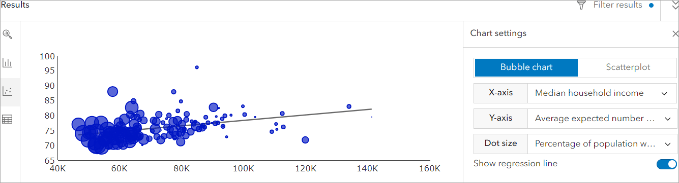
Another tool we can use in exploring the relationships within this data is a bubble chart. Bubble charts are a type of data visualization that represents data points in the form of bubbles on a graph. The placement of bubbles along the x and y axes signifies the relationship between two variables, similar to a scatterplot. The third dimension, represented by the size of the bubble, adds an extra layer of information, allowing for the comparison of additional data.
To access the bubble chart tool, on the chart settings, toggle the display to Bubble chart. Then, choose Average expected years of life from birth for non-Hispanic Blacks for the y-axis, Median household income for the x-axis, and use Percentage of population who are food insecure to determine the dot size. In this example, we noticed larger bubbles on the lower left end of the chart, indicating that areas with more food-insecure residents tend to have lower household income and reduced life expectancy.
Lastly, using the Table tab, you can export your data to Excel.
Conclusion
With Business Analyst Web App’s data visualization tools, exploring our data is now much simpler. The smart map search Results pane allows for comprehensive exploratory data analysis and visualizing trends in life expectancy across different race groups. By using several data visualization tools within the Results pane, we gain valuable insights, understanding not only the overall differences in life expectancy but also how various socioeconomic factors may influence these disparities across different race demographics. This process helps us gain a better understanding of the factors that influence life expectancy in the United States.
Data attribution
This article contains or references data from the following sources:
- Light Grey Canvas basemap provided by Esri
- County Health Rankings data provided by the University of Wisconsin Population Health Institute and the Robert Wood Johnson Foundation


Article Discussion: