The U.S. Census Bureau released block-level data on August 12th, 2021, in accordance with Public Law 94-171. Two weeks later, a feature layer with all 8,174,955 blocks was available in ArcGIS Living Atlas of the World, along with layer views for each state. Additional geographies (states, counties, tracts, block groups, etc.) were released shortly after, using the same processing methods. These layers are readily available to be accessed and used within typical GIS workflows or redistricting efforts throughout the country.
Understanding how to create layers such as these is useful for those who want to publish large feature layers on their own. Using ArcGIS Pro, ArcGIS Online, and the ArcGIS API for Python, any ArcGIS user has the power to share and map similar datasets containing a large number of records. This blog covers the high-level steps that the Living Atlas team took to create the 2020 Census Living Atlas items.
The goal of this project was to provide ready-to-use layers so that anyone needing Census data would not have to spend the time processing the data themselves. Another goal was to add value by making the final layers easy-to-use, even for those less familiar to Census products and documentation. To do so, the data attributes, boundaries, and documentation for each geography level all needed to live in one place: the hosted layer.
There were three major components: Pre-processing steps completed before the release, Data Processing steps to create the layers, and finally Hosting and Sharing steps including creating higher-level information products such as maps and atlases.

Pre-processing Steps
Before the data was released, we were able to read up on documentation and review previous decennial Census data to determine a process. This helped speed up the process once the data was released onto the Census website. These pre-processing steps also reduced potential for error down the line and increased overall quality and consistency of the final layers.
1. Process Boundaries
Before the Census releases the data tables, they offer their TIGER boundaries in File Geodatabase (FGDB) format. We grabbed the 2020 TIGER National Level Geodatabases in preparation for the data release because it can be done ahead of time. To prepare the boundaries for hosting, there are a few steps that were done at each geography level:
- Project the input from Global Coordinate System North American Datum of 1983 (GCS NAD83) to Web Mercator Auxiliary Sphere using the Project (Data Management) tool
- Repair the geometries to ensure no geometry problems exist with the boundaries. Both methods (OGC and Esri methods) are used in the Repair Geometry (Data Management) tool
When processing your own boundaries, consider using these steps so that your data is performant and can be used within analysis tools downstream.
2. Build Metadata
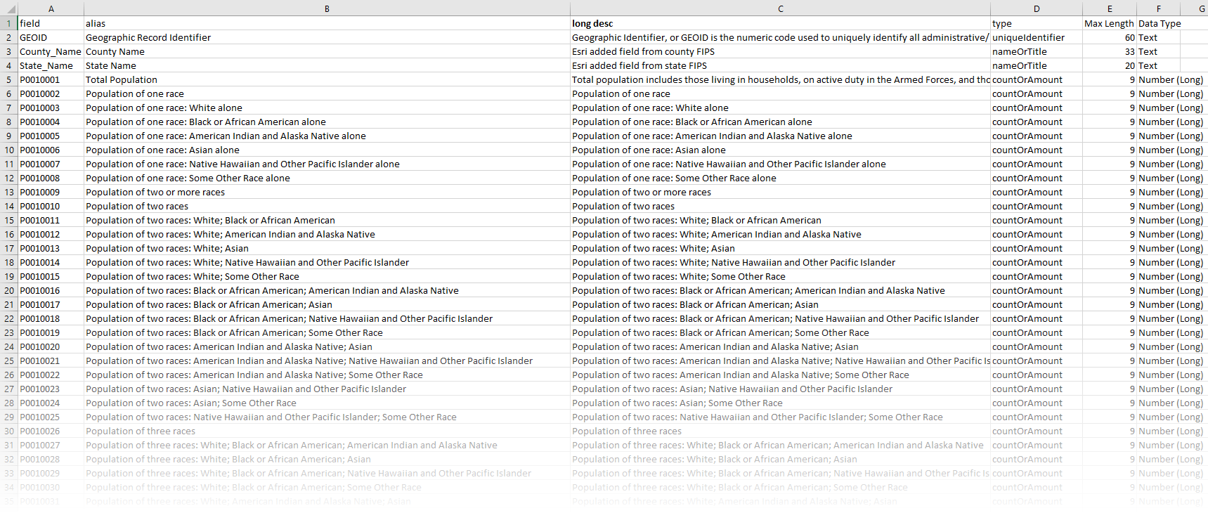
Census provides detailed information about the fields by defining the Headers for their legacy files. These specs were used to help determine the database structure for the final tables. The information was also provided in the technical documentation by geography. Using this information, we were able to define key metadata ahead of time:
- Field name
- Field alias
- Long description (detailed description of the field, normally found in a metadata PDF document, now provided directly within the map)
- Field type (string, short integer, long integer)
- Field length (if string)
This information was stored in an Excel table which was used downstream to help determine database and service structure.
3. Build Template Item(s) for Hosted Services
To create consistent documentation and to allow for automation, we created a template item details page for our hosted services. We created a blank item in our ArcGIS Online content and built the item page as we wanted it to appear for all Census 2020 items. Anywhere within the page where the items differ (the title, geography level, etc.), placeholders were specified. For example, geographyType was used as a placeholder for the geography level, e.g. states, block groups, or tracts. Later in the process, a python script was used to fill in all placeholders and the item page/REST endpoint details were automatically generated based on the template item.
This type of workflow is ideal when working with a large number of datasets that need to be hosted. If there can be a common template to communicate the metadata, this method can save the time of hand-creating each item page. It also ensures that the REST endpoint is updated for those who access the data through that interface.

Data Processing Steps
Once Census released the data via FTP, the following steps could start. We did do some prep work using 2010 data to test these processes when possible.
4. Tabular Data Transformation (via SAS)
Downloading the source files from Census in the form of state-level zipped files is just the first part. Transforming those into the final attribute tables takes some tabular data manipulation. This step can be done using a variety of tools: Python, R, SAS, Microsoft Access, and more.
We chose to do it using SAS, which allowed us to take advantage of the import scripts that Census provides. Our SAS program does the following:
- Unzips all states’ zipped files and stacks them into one national file
- Extracts out each geography level of interest, joins the six tables and the Header table into one wide table
- Adds in State_Name and County_Name fields when appropriate from a lookup table
- Reorders fields, drops unnecessary fields from the Header table, and calculates additional fields with some QA checks
- Exports an attribute table for each geography level to CSV, as well as exports a fields list
5. Convert CSV to Table
CSVs can be tricky because they don’t have specific field types or structures defined. To overcome these factors, ArcGIS Data Interoperability tools were used to convert the SAS outputs into ArcGIS-ready tables. These tools allowed us to specify factors such as the database structure and the field types.
The general workflow used the Data Interoperability Extension to read the CSV, define the schema, and output to a table. Using the specs from #2 above, the schema was designed ahead of time. Before-hand, testing was done with 2010 Census data to test the process and outputs. When the new 2020 Census data was released, it was funneled directly into the tool using the 2020 specifications and data. The Data Interoperability tool allowed us to confirm the number of records matched the tables from Census, and solidified the table schema ahead of time.
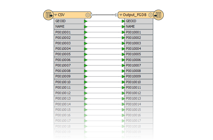
When working with datasets with a large amount of rows, the Data Interoperability tool allows you to define schema and ensure all records are accounted for. This reduces the risk of lost records.
6. Join Table to Boundaries
Using the Add Join (Data Management) tool, the output tables from step #5 were joined with the boundaries prepped from step #1. The Add Join tool allowed us to validate the record count before running the join in order to confirm no features were lost during processing. To speed up the join, an attribute index was added to the GEOID field on both inputs before the join was run. This can reduce processing time when working with large datasets such as 8 million Census blocks.
Once joined, the data was exported to a new feature class using the Feature Class to Feature Class (Conversion) tool. The Field Mapping allowed us to control the order of the fields so that the data values appeared before the boundary-specific fields such as Area Water or the Latitude/Longitude.
To finalize the data, the geometries were repaired again (using both methods), and an attribute index was added to the GEOID field. These small details ensure that the data will work well and fast in downstream analysis/mapping.

Hosting and Sharing Steps
7. Host Data to ArcGIS Online
To host the data to ArcGIS Online as a hosted feature service, each geography level exists in its own File Geodatabase and is zipped. From My Content, the zipped File Geodatabase was uploaded to ArcGIS Online so that the raw data would be accessible for those who need it. From the File Geodatabase item, a hosted service was published.
A few benefits for using hosted services on ArcGIS Online:
- ArcGIS Online hosted layers are useful when you need to expose a map or dataset on the web but do not have your own ArcGIS Server site. It’s also an easy way to share certain maps with an internet audience if your own ArcGIS Server site cannot be made public.
- The layers are hosted in Esri’s cloud and scale dynamically as demand increases or decreases.
- You can easily customize and manage your services through the My Content interface on ArcGIS Online, keeping all of your content organized and in one place.
8. Document Hosted Services
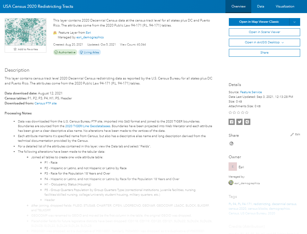
To make the data easier to understand, the detailed field information from step #2 above was applied to the service and item using Python. The field alias, long description, and field data type were applied. To apply metadata to the the items as they were created, a Python script was run to update the items with detailed documentation. The script used the template items from step #3 above and generated item details pages which were applied to the item page and the REST endpoint. A similar update method was used to update some item page settings:
- CDN was set to 1 hour to optimize the layer’s performance
- Delete protection was turned on for each item
- The ability to export the data was turned on
This script or this tool can apply similar alias names to your services/tables.
Detailed item pages and alias names help communicate information to the end user of a data source. When making your own services, these best practices allow for transparency, and encourage others to use and understand the data. These details also empower your services to qualify as Living Atlas content, which is required to be well-documented.
9. Configure Services
How many times have you opened a dataset and you saw blank polygons? To avoid an empty map, the layer has default symbology configured around the core concept behind P.L. data: the population. The symbol faintly shows the outline of each polygon for reference, but the focus of the map is on the population count. Areas with no population have attribute-driven transparency to focus the map on populated areas, but these features can easily reappear if you need them by removing the transparency or changing the attribute being mapped.
If you click on a feature, you’ll notice a pre-configured pop-up. This helps provide important information with a single click. This information can also be customized to your needs by configuring the pop-up. What you see within the default pop-up is a summary of key details about an area. At the tract, block group, and block levels, the pop-up aggregates information from the surrounding polygons to help address differential privacy concerns. An Arcade statement was used to summarize nearby polygons for this method.
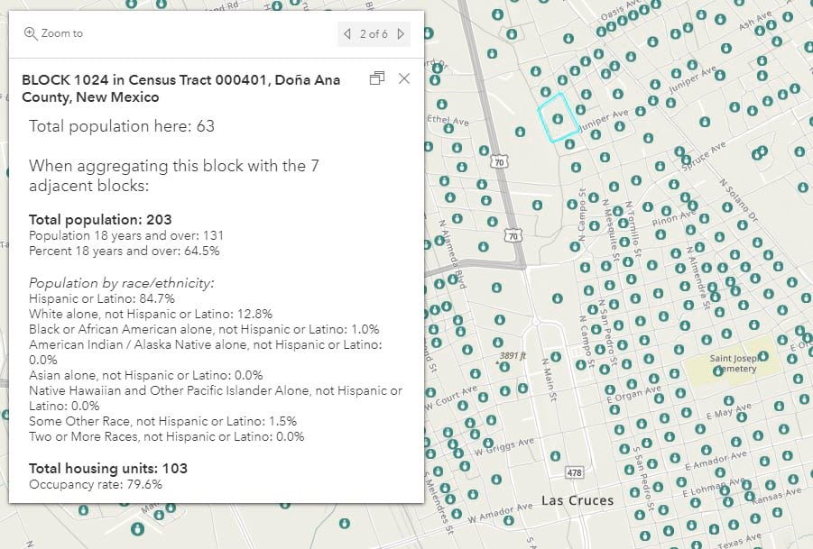
Setting symbology and popups is part of making a layer “map-ready” compared to a bare REST endpoint. This helps the map reader/creator understand the data more quickly, and allows them to easily customize the to their needs.
10. Create Views for Each State
Redistricting data is commonly used at the state level to help determine new Congressional District boundaries. For this reason, the block-level data was also offered at the state level using feature layer views. This technique is handy for working with large data that you also want to share at more local levels. Views create a separate layer ‘view’ of the original service, allowing for a smaller, filtered subset of the data for a different audience. While each view gets its own unique REST endpoint, the data is only hosted once, reducing the amount of storage needed to reach additional audiences.
11. Create Maps and Apps
So far we have seen how the layers were created. Layers are the building blocks for great maps, which is why there are many ready-to-use web maps that are available using the 2020 Census data. Web maps, unlike layers, store information like the basemap, bookmarks, and other customizations which can be handy for sharing spatial data. Web maps are also a key component for creating things like story maps, dashboards, or instant apps.
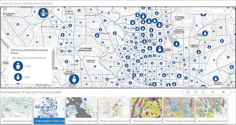
The Living Atlas Policy Maps team created dozens of web maps from this dataset, each visualizing a specific topic within this vast amount of data, for example, Total Population 18 and Over, and Housing Vacancy Rates. Each web map is available in Living Atlas for you to use in your own apps, story maps, dashboards, hub sites, or websites.
We also created some focused web apps highlighting some of these maps. The most comprehensive one is simply called Census 2020 Atlas of Redistricting:
Others are more focused on a particular subject, such as Census 2020 Atlas of Race Alone or in Combination, which includes those who are multiracial in each racial group they identify with.
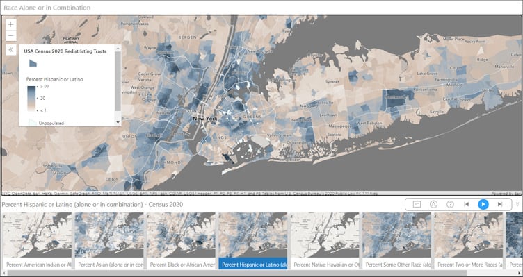
These two atlases use the Portfolio Instant App to showcase multiple maps, however, other Living Atlas apps that highlight maps from Census 2020 redistricting data use other types of Instant Apps, including Media Map and Chart Viewer.
We even used a few of these maps to build a new collection available on the Esri Maps for Public Policy site. Search for your community, and share the collection of maps with others through email or social media with one click.
Taking the time to ensure quality throughout the layers paid off, as it greatly reduced the effort need to make these maps and other information products.

Use These Living Atlas Items
Living Atlas items work throughout the ArcGIS suite of products. Pull in the national layers or state layer views into Pro and Insights. Put a particular one of the maps you like into a story map or instant app. Showcase one of the Living Atlas apps in a hub site or web experience. Take it one step further and modify these maps and apps to fit your own needs, or start by creating your own map. You can also export the data to various GIS formats or perform analysis on them as-is.
Working with Census data is no longer expensive or cumbersome. We understand that many of you want to combine this data with your own organization’s data, which may be equally large. The layers are exportable, available for analysis, and FGDBs are also available.
Use These Processes to Publish Your Own Data
All the workflows discussed here can be done using a combination of Python, ArcGIS Online, and ArcGIS Pro. As a layer publisher, you can borrow any of these steps that make sense for your project’s needs. Whether it’s building out field metadata ahead of time, or creating views for subsets of your data, something from our process listed here may spark some ideas for your own work!


Article Discussion: