The Challenge: You have a pretty big table of data with location in it and you want to make a striking visual for a presentation or press release that shows a specific geographic trend. You have no access to ArcGIS Pro, or you’ve never heard of it.
Could be:
- Your organization just invited you to a thing called “ArcGIS Online”
- You have it (for free) in K-12 classes or Nonprofit organizations.
- You’ve been invited to be a Hub Community member by your city.
- Your University has it, and you get a login as a student
- You’re just curious. Awesome! Fully functional free trial right here.
If that’s the case, welcome to GIS! Let me show you around! You’re going to make a scene, and I mean that in a good way. We’re starting in 2D and taking it to 3D.
If you’re a GIS professional, you’re cool too. You can do this in ArcGIS Pro, but maybe you’re on an iPad or someone else’s computer. Maybe this inspires you to do this with Notebooks!
We’re going to go through a couple of steps:
- We’re going to convert that table into a feature by using the location data in that table to put the points where they are on a map. This is called geocoding.
- We’re going to make a grid to count the points in. This is called a tessellation.
- We’re going to count those points in each grid cell. This is called aggregating points.
- We’re going to make sure the count translates well into a vertical height.
- We’re going to turn this 2D grid into a 3D visualization with extrusion.
- We’re going to save this and share this for the world to see your 3D scene.
Let’s get started!
The first thing is logging into your ArcGIS Online Organization and clicking “Map” at the top.
I have this SampleAddresses.csv file for you to try this with. Download it, and find where you’ve downloaded it to.
Geocoding
- With your starting map up, drag the SampleAddresses.csv file into your map.
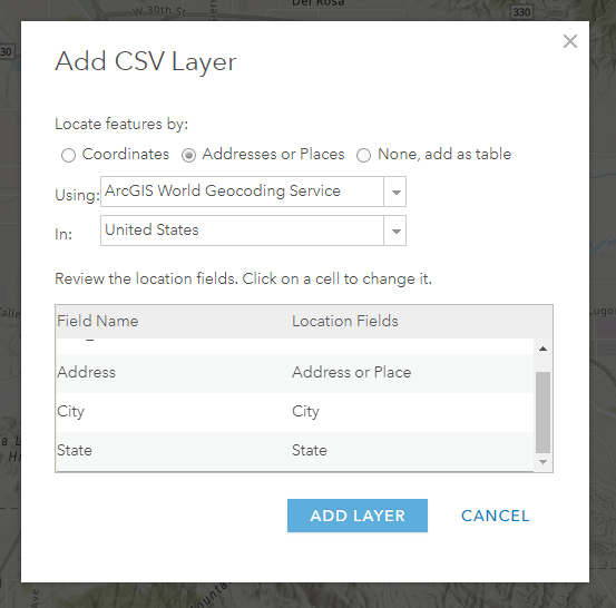
- The map viewer recognizes that you’re trying to add this csv, and starts lining up geocoding information. It identifies that you’re trying to add addresses, and if the fields are named appropriately, it’ll line those up to geocoding services. You’ll get more accurate results if you set the country that this data is set in (in this case, this is in Redlands, CA in the United States). Click “Add Layer”.
*Note: You can drag and drop a layer with less than 1000 entries into the map viewer, if there’s more than 1000 entries, you’ll need to add the CSV in “My Content.”
3. This data set has Addresses with City and State fields separated, and you’ll find that it geocodes to the map and then attempts to symbolize the data with smart mapping symbology. For “Choose an attribute to show”, select “Show location only.”
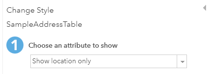
4. Hit “Done”
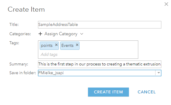
5. You’ll see SampleAddressTable in the Table of contents in the left side. Click the ‘…’ on the feature and “Save Layer” on the bottom of that dialog.
6. You’ll be asked for a title, tags, summary and folder. This is required information about your saved layer.
7. Congratulations! You geocoded the table and you now have a point feature layer.
Create tessellation
In this section, we’re going to create a grid (a tessellation) to count the total number of points within. We’re actually going to create a tesselation out of hexagons because they tend to look and work better for summarization.
- Zoom into the area that you want the grids created over. The next tool will use your display extent to define the coverage of this tessellation.
- Click Analysis> Manage Data> Generate Tessellations
- Choose Shape: Hexagon
- Define Extend: Same as display
- Define bin size by specifying: Choose Distance and set 500 meters
- Name the Result Layer name and set saving location
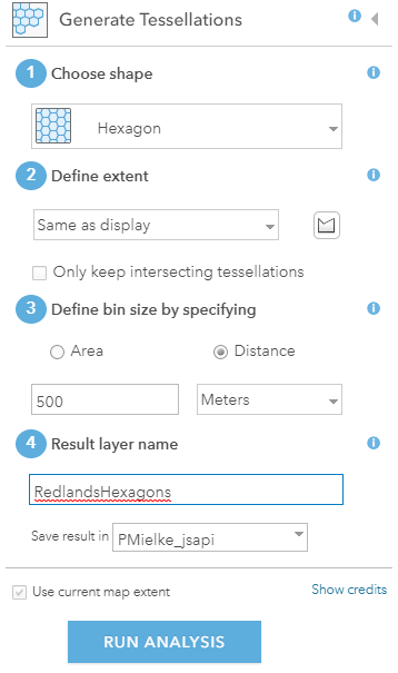
3. Click Run Analysis.
*Note on credits: There’s a ‘Show Credits’ button next to “Run Analysis” that will tell you this will consume around 1 credit. This is a nominal fee associated with the analysis transaction, and it’s built into organizational purchases. It’s about the cost of photocopying a single page at a copy store. There’s a lot of capability in ArcGIS, and it’s meant to be used. Just be aware of what you’re asking for before you photocopy a library. Read more here.
4. You have hexagons all over your map now. Good! GIS folks call them ‘hex bins’. Onto the next section!
Aggregate Points
Now you’re going to count the points inside of the hex bins, so that there will be a field in the hex bin attribute table with the count of the points that fall inside of each bin.
Wait a minute. Looks like there are points that are hard to tell which hex bin they get counted in- What if they fall on the line? Are they counted in both? Interesting, but there is no such thing. Points and lines have no area, and they cannot overlap each other. If you’re into that, it’s good to introduce you to the Modifiable Areal Unit Problem, as it does play a factor in approaching this kind of analysis.
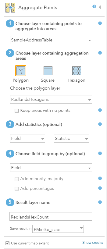
- Click Analysis, Summarize Data, Aggregate Points.
- Fill in these values in the analysis dialog:
- Choose layer containing points to aggregate into areas: SampleAddressTable
- Choose layer containing aggregation areas: Polygon (and the layer you just created: RedlandsHexagons). You can actually generate the tessellation directly within this tool, but it’s good to know how to complete the previous step.
- Uncheck “Keep areas with no points”.
- Add statistics(optional). These will remain blank. If your address table had numeric data that you wanted summarized (money donated, for example), you can summarize that data here.
- Choose field to group by (optional) will remain blank.
- Result layer name: RedlandsHexCount
- Click “Run Analysis”
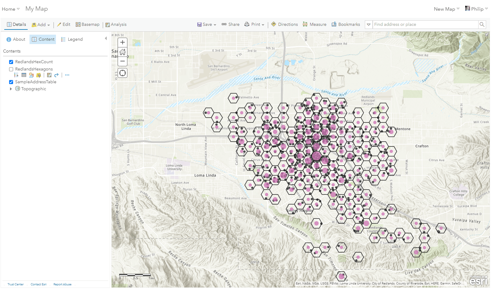
You should have something that looks like this. Uncheck Redlands Hexagons and look at the result. The “Count of Points” field in RedlandsHexCount has been automatically symbolized with smartmapping.
Prepare for Extrusion
Now you have hex bins with a count of points that fall inside of them. There are 188 features that are almost ready for 3D visualization. Just one catch- these counts must translate to a unit of measurement for height. The hex bin with the highest count has 53 points that fall within it. If this were 53 meters tall, that hex bin’s height would be very small compared to the known width of 500 meters. Let’s change that by adding a field and calculating a new value to extrude on.
- Click the “…” on RedlandsHexCount in the Table of Contents of the Map Viewer.
- Click “Show Item Details.” This is ‘the guts’ of the data you created in earlier. We’re going in.
- Click “Data” on the blue bar.
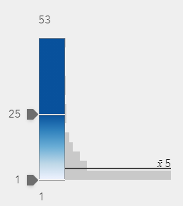
- We’ll look at the statistics on the “Count of Points” field. Click on that field and click “Show Detailed View.”
Take a look at the Summary. You can see a range from 1 to 53, and the bar chart displays number of features within that class or group. Mousing over the Greek characters, you can see that the average is 5.149.
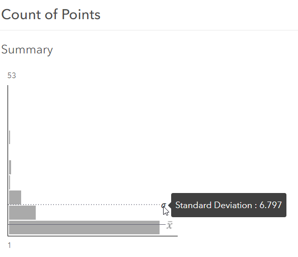
This graph is telling us that out of the 181 hex bins, many of them are low counts. Keep this distribution in mind when calculating an Extrusion Height field.
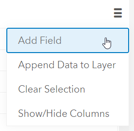
6. On the right of the table, you’ll find an icon with 3 lines. Click that icon and click “Add Field”
7. Enter “Height” for the Field name and Display Name, and Important, select “Integer” for Type.
8. You’ll now see “Height” in the table. Click that field and select “Calculate”.
9. ArcGIS Online give you the option for language used in the calculation. Select “Arcade.”
10. You’re going to calculate a vertical unit height that makes sense based on the distribution of the “Count of Points” field values. How tall should they be? This may be something that you have to try a couple of times to get right. The average is 5.149, and 500m is a good height for average values, given the known horizontal size of our grids (500m). Multiplying the counts by 100 should give good results.
11. In the Arcade Calculator, click the arrow next to $feature and click $feature[“Point_Count”]
12. Type “*100” (That’s an Asterix, which signifies ‘multiply’)
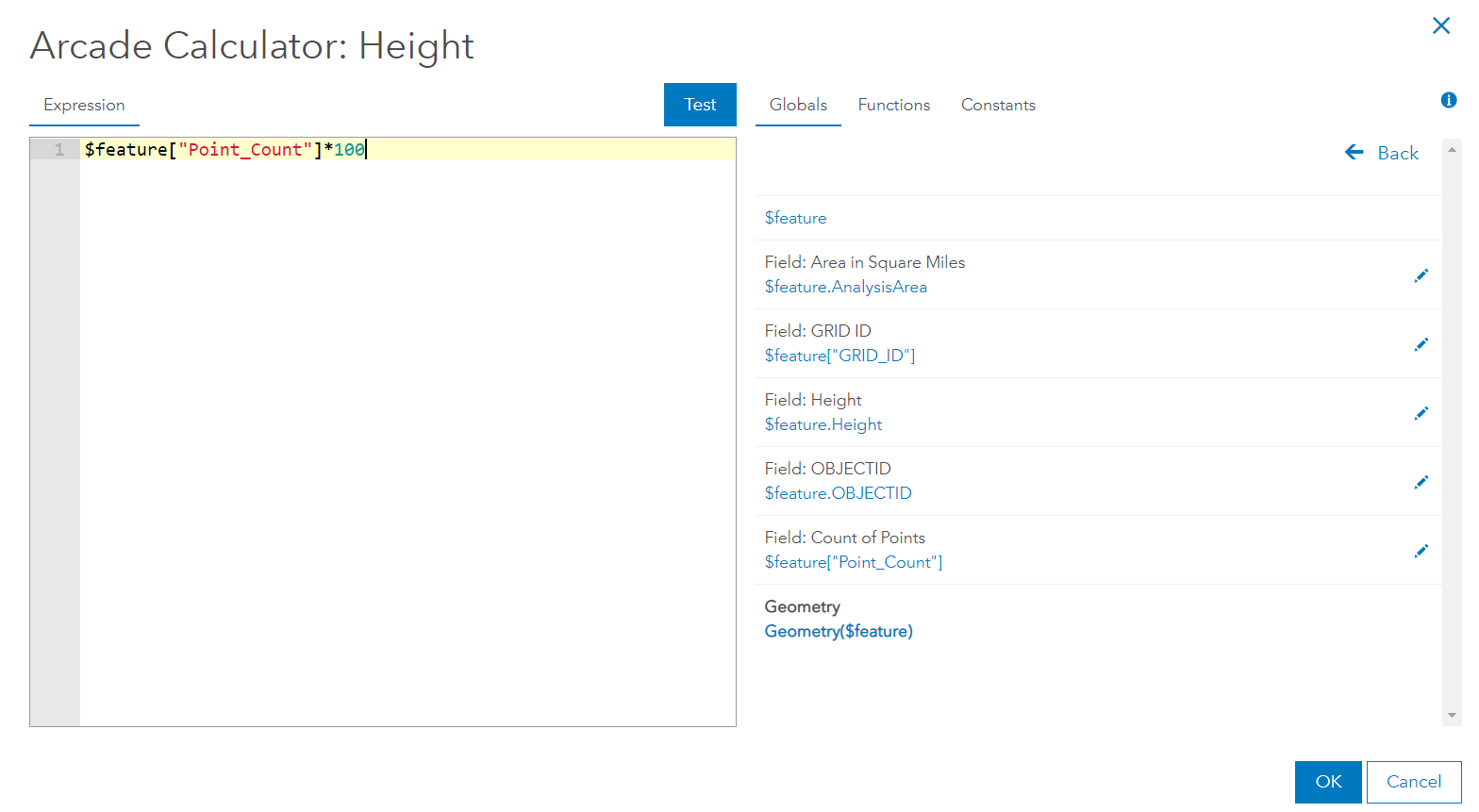
13. Click “OK”. You should see it process the data and now see values in the Height field.
14. Now, on the blue bar, click “Overview”.
15. On the right of the Overview page, click “Open in Scene Viewer”
Extrusion styling in Scene Viewer
You’re now going to style the data and create a scene in Scene Viewer, the 3D web viewer for ArcGIS Online. You’ll use “3D Counts and Amounts” smartmapping styling to color the hex bins based on the “Count of Points” field, and you’ll extrude the hex bins with the “ExtrusionHeight” field. This may be a bit of an introduction to Scene Viewer for you, so if you’d like to learn some of the basics, check here.
- On the “RedlandsHexCount” feature in the table of contents, click the three dots to the right and click “Layer Style”.
- The “Choose the main attribute to visualize” should have automatically selected “Count of Points”. If not, select that.
- Click “3D Counts and Amounts”
- Click “Options”
- You want to draw attention to higher values, so drag the upper value up and see the coloring of the features immediately respond to these change. Drag that to 25 (or type it).
6. On Height, click the dropdown menu and select the “Height” field you calculated earlier.
7. Click “DONE” and “DONE” again.
You can experiment with turning edges on or labelling in the previous dialog, but this works well for this.
This is a thematic scene, and you must take how you display elevation under consideration. You’ll notice, looking at this scene, that hex bins start their height on the ground. When the ground has hills and mountains (as Redlands does), the significance of height is a little confused by varied elevation. You should remove elevation with the following steps.
8. Click the arrow next to Ground.
9. Click the three dots next to “Terrain3D” and click “Remove”
The ground is now flat, and it doesn’t confuse the meaning to the data you’re portraying.
10. On the righthand side, you can change the basemap you’re using. I like Nova Map for this kind of scene.
Now you’ll save a few slides to save the camera viewpoint.
11. Click “Slides” on the bottom left.
12. Navigate to a good point of view and click the “+Capture Slide.” Repeat until you have a few useful slides to show your scene.
13. Click “DONE”
14. Click “SAVE SCENE”
15. Give your scene a Title, Summary and tags
16. Click the Share button
17. You’ll see a warning that this scene is not shared with the public. Click “Change Share Settings”
18. On the right of the Overview for the Scene, click “Share”. Select “Everyone (public)”. It’ll also ask you to update permissions for the “RedlandsHexCount” feature.
19. Go to the browser tab with the scene and click the “Copy to Clipboard” icon next to the link
You can now share this link and the viewer will be able to open this scene in Scene Viewer. This is a great start if you want to incorporate this into a 3D configurable app, Web AppBuilder, Experience Builder or Storymaps.

Article Discussion: