
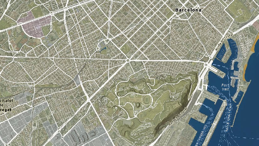
One of my favorite ways to style maps is with the Vector Tile Style Editor. What’s so wonderful about it is that you can take things that you like from one Esri basemap and join it with another. For example, check out this map which is the Esri World Imagery and World Topographic Basemap mixed together.

This hybrid approach allows the best of both types of basemaps. You get the context of reality while subtracting out everything else with a simplified digital representation.
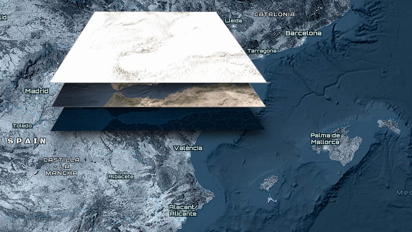
The way this map was designed was at the global scale, the land is masked out by the Topographic Map. Then as you zoom in, the beautiful World Imagery is revealed using opacity driven land and vegetation layers from the Topographic Map. This allows the basemap to be in a good position to have other data placed over it (Note for a good working example, this is how the basemap for the Wildfire Aware app was created).

While working on the map above, I came across another visualization that I thought was really intriguing. Check out what happens when you combine World Contours and World Imagery, it looks like it was outlined with a pen by a terrain artist. These contours help accentuate the land very elegantly. They don’t come on until 1:72,224 and then wow! It’s like the depressions and cliffs come alive! I’m seeing things that I don’t normally see in the imagery and I really love that.

How to do this?
Start by signing in with the Vector Tile Style Editor. Click on the top right green button for “+ New Style” and scroll almost to the bottom and select the World Topographic Map (with Contours and Hillshade).

When it opens, click on the icon for Edit Layer Styles.

There is a list of different layers that comprise this basemap. Expand some of them and you can see that there are nested categories of layers for customization (polygon fills, lines, fonts, and sprites).

For our purposes we are only interested in a few layers that are found within Natural, Land Use, and Water categories. You could use the Editor to go in and turn off all of the unneeded layers one by one, but it’s faster to remove them directly from the code using the JSON editor.

For this workflow, I find having a Notepad++ document (or other text editor that keeps the JSON formatting intact) helps to keep me organized. It also allows you to backup the code when done. If you prefer, you could also do this within the code editor by deleting what you don’t want.
For this map the only layers we are interested in from the Topographic Map are:
Natural – Hillshade, Land, Vegetation, Forest or Park, Contours
Land Use – Park or farming
Water – Ocean, Bathymetry, Lakes
This ends of being 1,249 lines of code ending on “Water area/Lake, river or bay”.
What we are going to do is copy/paste the sections of the code we need and put them into the Notepad++ document. Let’s start at the top by copying all the Hillshade layers plus the beginning JSON formatting. This is line 1-113.

Next paste that section of code into a Notepad++ window. You should end with “Hillshade/Shadow Very Strong/1” at the bottom when you get it all in, and mind that you to get the comma you see on line 113. This helps to keep the formatting consistent as you go through it.

It’s the same workflow for all of the other layers required – copy and paste each section of the code that’s needed and place them in a Notepad++ document until everything is there. This will take some time and attention to scan through the code and find everything you need.

Once everything is there, double check the formatting. Next copy the entirety of the “new” code from Notepad ++ document and then paste it back into the JSON Editor and Update it. If the code doesn’t work, check the code for errors. You might be missing a comma or brace. To double check, you can download the completed code here.

Now this basemap contains only the layers we want.

Save this as a new Vector Tile Layer in your account.
Styling
Let’s walk through the visualization settings for of each of the layers.
Hillshade: This layer is an awesome addition to our options for terrain visualization! As customizable vector tiles! For this map the default colors were kept, but their opacity was adjusted for every layer, so that it goes from 25% opacity at “0 Zoom” to 0% 0pacity at “11 Zoom”. This layer certainly adds texture to the map and embellishes the mountain areas; however, when you zoom all the way in at Scale 11 and just want to see the pure Imagery it disappears. Take note that the Hillshade layer also covers the Ocean and Bathymetry layers and there is more on that later.

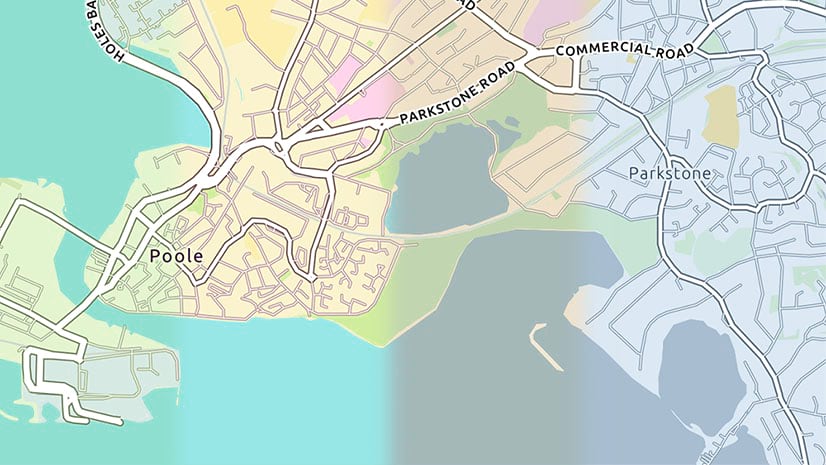
Land: The Land/Not Ice layer has highly customized opacity. It starts off at the global scale as a sold white. Then as you zoom (and you want to see more of the imagery) the opacity lowers until at Scale 18 it is at 0%. Using the land layer to soften the imagery is a good way to get the best of both worlds.

Vegetation and Land Use: These were all treated with varying shades of green. Their opacity adjusts as you zoom in and out of the map. This layer starts to come on very slowly at Scale 5 by design. If it came on any earlier it would be too distracting. Its main purpose for this map is to tint the natural and forested areas with more green. This adds a bit of drama especially in the mountainous areas.

Contours: These were probably the trickiest of the group to wrangle. The color needs to stand up to the imagery no matter where you are on the earth, so a dark brown was used that gets even darker as you zoom in. The stroke size was adjusted as well so that they are 1.0 moving to 2.5 to 3.5 pt depending on what scale you are. There is also a heavy blur of “2” set for the lines so that they appear on the map more organically.

Ocean: Let’s see what it looks like without any additional layers.

While absolutely beautiful, I can’t stop looking at it because of that. Let’s tone it down a bit so it’s part of the story and not the entire story.
Let’s start along the coasts. For the areas surrounding the land (Depth 1 Bathymetry) a medium blue was used along with opacity starting at 30% going down to 10%. Now these areas pop a bit, but not too much.

Bathymetry: This will be a surprise, but the bathymetry is actually gray in color with only 10% opacity. Remember I mentioned earlier about the Hillshade classes covering the Ocean and Bathymetry layers? The first three (Hillshade Shadow Base 1, Hillshade Highlight Light 1, and Hillshade Shadow Light 1) do faintly play a role here. This affects the visualization. However, by adding in the gray over it (which is tinting the bathymetry darker) it allows for more of a range of color. Look how the palette is without the imagery:

Now here it is along with the imagery. This 10% sequential gray palette tones out even the highest values of the imagery and allows the texture of the bathymetry to still come through.

Lakes: These need to behave similarly to the ocean but since they are most often surrounded by land, they got a slightly lighter blue with 100% opacity. This is another way to adjust your layer and how much presence it gets on the map. It starts at 100% and then by Zoom 13 it disappears.

The final step is to open up an ArcGIS Online webmap. Replace the default basemap with this customized Vector Tile Layer along with World Imagery. Let’s bump up the Imagery layer with the Saturate Effect by setting that to 130. This gives it a bit more richness and helps to play off the contours.

Want to bump it up even more? Add in World Hillshade and use the Blend Mode Multiply and give it 25% Transparency.

Here’s the webmap and it contains bookmarks of the places shown in this blog. There is also a final vector tile you can retrieve to compare with your own, and also the code used in this blog, shown in detail.
Another idea not shown here is to add the layers to a 3D Scene and then really have some fun…like how Halfway Hollow in Utah looks.

Resources
Since the final product was displayed at the beginning of this blog article it only seems fitting to end with resources, of which there are a ton!
Everything you need to know about Esri Vector Basemaps from legendary basemap cartographer Andrew Skinner. Below are three blog articles that expand on many of the things discussed here.
Humorous video by Tommy Fauvell and John Nelson about Advanced Vector Tile Style Editing as well as another blog article by the pair that digs into what we talked about here.
Documentation about the Vector Tile Style Editor and here’s one about creating your own vector tiles which you could then use in the Style Editor!
Please reach out to me with comments or questions!


Article Discussion: