ArcUser
Fall 2011 Edition
Making Connnections
Modeling the relationship between food, energy, and environmental impacts
By Todd J. Schuble, Esther E. Bowen, and Pamela A. Martin, University of Chicago
This article as a PDF.

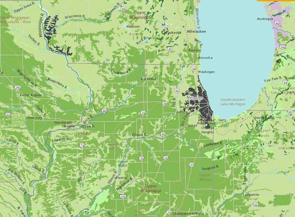
The foodshed mapping project explores the potential for foodshed development in the upper Mississippi watershed, including the Chicago metropolitan region.
Researchers at the University of Chicago are employing geospatial analysis to quantify the resource potential for establishing foodsheds, increasing regional food production, and assessing impacts of that food production on health and the environment.
Feeding the City
Grouped under the heading Feeding the City, projects examine energy use and greenhouse gases associated with small-scale sustainable agriculture on both rural and urban farms and the potential for foodshed development in the upper Mississippi watershed, including the Chicago metropolitan region. The research team that worked on foodshed mapping included the authors of this article—Todd J. Schuble, Esther E. Bowen, and Pamela A. Martin—as well as Sabina Shaikh, Julia Govis, and Eugene Yan. Primary funding for the foodshed mapping project came from the University of Chicago's Energy Initiative.
Foodshed Mapping
Calculating a foodshed is a simple process. A foodshed is the amount of land necessary to support a population's food needs. A handful of variables are used to compute this model: the amount of food one person requires, the total number of people that need to be fed, and the amount of available land necessary to produce the food.
The United States Department of Agriculture (USDA) provides two major inputs for the foodshed calculation. The first input is the average caloric intake of an adult resident of the United States. The second input—more important to spatial analysis—is data about soil from the Natural Resources Conservation Service (NRCS) Soil Survey Geographic (SSURGO) database. This data includes vector polygon boundaries for different soil types along with soil and land-use attributes for nearly every county in the United States.
Python scripting was used extensively in the project to modify and prepare the SSURGO data for analysis. For each county in each state, SSURGO provides an individual file. The county file contains two directories for spatial and tabular data in addition to the metadata files. The spatial directory contains point, line, and polygon shapefiles delineating areas of contiguous soil types. In the tabular directory, attributes for the soil features are stored as text files.
The United States Department of Agriculture Natural Resources Conservation Service Soil Survey Geographic (SSURGO) data, available from ArcGIS Online as a map and a map service, was used in the project.
The attributes in each text file are joined to the corresponding soil features using a unique identifying code. The text file naming convention that was implemented gives each file a unique name so processing can be automated. For example, _il001 was added to the mapunit.txt file for Adams County, Illinois, which results in a unique file name of mapunit_il001.txt. Attribute text files do not include headers, so before joining them to the soil features, headers are added to text files of interest according to NRCS metadata standards. Of the 24 attribute columns in each mapunit file, the farmlndcl and mukey columns were retained and joined to the soil layer using the mukey field.
The US Census Bureau provides two more pieces of data for the equation: individual urban area boundaries and total population for urban areas represented as vector polygons as delineated by the US Census Bureau 2008 TIGER/Line files for US states (US Department of Commerce 2008).
Finally, transportation must be accounted for. In this model, only road transportation data was used. Esri's StreetMap Premium for the United States and Canada included vector line data for every street in the study area as well as posted speed limits for each street segment. This information is crucial to determine travel times from urban area centers to the individual soil polygons where food is produced. Other versions of the model include rail and water transportation modes as well.
Foodshed Model
Beyond the spatial data necessary to calculate the foodshed, these four assumptions are included in the foodshed model calculations:
- All persons in the study area eat the same daily average number of calories as calculated by the USDA. According to the Agriculture Fact Book 2001–2002, the aggregate food supply in 2000 provided 3,800 calories per person per day with about 1,100 calories being lost to spoilage, waste, or other losses. The caloric intake of individuals is, of course, very different. However, using 3,800 calories as a base simplifies model calculation.
- The NRCS classifies soil in different ways. Some examples: prime farmland, prime farmland if drained, and prime farmland if irrigated. The model only includes soil classified as prime farmland or farmland of statewide importance in the analysis. The model assumes these selected soil types would produce the same yield regardless of location despite the fact that different soil types obviously produce different yields depending on meteorological factors along with human intervention such as fertilization or irrigation. However, for this model, all yields remain equal regardless of farmland type designation.
- The model's population base consumes only two types of foodstuffs: grains and vegetables. Different food types and groups provide different calorie amounts. In this model, all grains and vegetables have the same caloric output. In subsequent variations of the model, calorie amounts vary by crop type, and animal-based products (dairy, meat) enter a population's food pyramid. These additions expand an urban area's foodshed, because growing varied crops or animal feed requires more land.
- As previously stated, all soil types in the model produce the same yield regardless of crop type. Therefore, every acre of land produces the same number of calories. This standard produces the foodshed person-to-acre ratio. Consequently, the acreage necessary to fulfill a population's caloric need is calculated through simple multiplication.
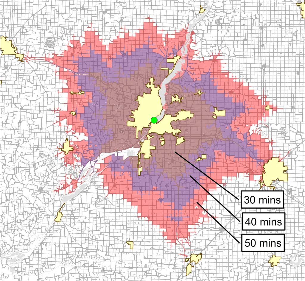
Different time intervals define the service areas until threshold acreage is captured for the urban area's population.
Since the threshold acreage to feed an urban area's population is known, the remaining unknown is the time buffer that will define the boundaries of the foodshed. The time buffer is the minimum amount of travel time necessary to capture the threshold acreage for an urban area.
ArcGIS Network Analyst creates the time buffer. A service area layer (or time buffer) is defined using the StreetMap Premium data and a predetermined default break value for the service area. In this model, the service area's starting default break value is two minutes. Measuring along the street network for two minutes in all directions from the centroid of an urban area creates the initial service area layer. Next, a simple Select by Location function executes to determine if the necessary number of acres (soil polygons) for the urban area exists within the service area layer boundary.
If the threshold acreage is not met, the routine deletes the layers and continues to loop, doubling the default break value (or time restriction) with each iteration until the acreage summation within the service area is greater than the threshold acreage. Once the model goes beyond the threshold, the last default break value used is divided by two.
The model then multiplies the last default break value by 1.5 (instead of 2) until the acreage summation within the service area is again greater than the threshold acreage. If the total acreage is too much, the last default break value is divided by 1.5, and the product is then multiplied by 1.25. This process continues overshooting and dialing back the default break value at lower and lower rates (e.g., 1.25, 1.125) until the minimum default break value captures the smallest number of acres necessary to meet the threshold acreage of the urban area.
Once the optimal acreage that meets the threshold value is achieved, the selected soil polygons are tagged with the urban area's name in the attribute table. This prevents other urban areas from including those polygons for its foodshed. The model then begins the entire foodshed definition process again by moving on to the next urban area in the region.
Urban areas that are in close proximity may have overlapping foodsheds. However, in this model, no two urban areas can share the same land in their individual foodsheds. To address this issue, a network accessibility index is calculated for urban areas within the region. The less accessible an urban area is, the more priority it receives in choosing land within its proximity. Two variables define the accessibility index: the number of connections that intersect an urban area and the capacity or speed of those connections. Through this process, foodsheds for very large urban areas may surround smaller, previously designated foodsheds but will not share the same land.
The complexity of the foodshed model increases with the size of the region being analyzed. Since all SSURGO soil vectors from each county are merged into one seamless vector dataset, the number of records being processed for a foodshed becomes staggering. The largest model run to date includes soil and urban area data from 12 states in the Midwest. This model encompasses 827 urban areas and approximately 15 million soil polygons.
Models and datasets of this size have been processed in the past using grid computing. However, this model proves that large-scale vector data processing is not only feasible but also relatively easy. This model produces output at an extremely high resolution with pinpoint accuracy. Moreover, processing is comparatively quick.
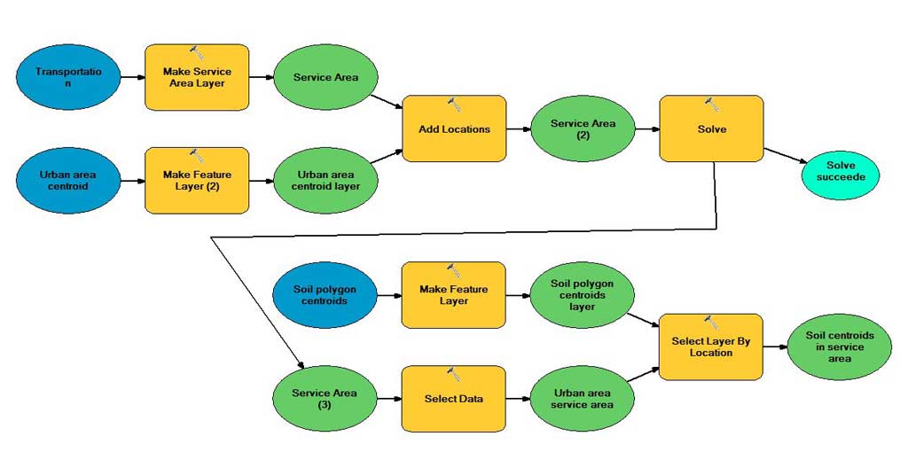
The functional flow model serves as the basis for calculating the foodshed.
This foodshed model processes all data using a simple Python script embedded with ArcGIS functions for the spatial queries. The back-end infrastructure for the process model includes a robust relational database and database server. The data is stored in a PostgreSQL database with ArcSDE 10. The database server specifications are relatively powerful but not extravagant: the server is running on a Red Hat Linux 64-bit platform with dual quad core 2.66 GHz Intel Xeon processors and 12 GB of RAM. With these specifications, the 12-state model ran in just under 60 hours. There is still plenty of room for this model to improve in terms of speed, agility, and complexity.
A Strong Start
The foodshed model as described here is incomplete but provides a very strong working base. Many of the omitted variables mentioned previously, such as different transportation modes, crop variation, yield variation, and meteorological factors, are currently being integrated. The model continues to be improved with the addition of better processing infrastructure and more variables.
The goal is to build a foodshed model that can emulate the environmental and economic conditions as closely as possible, not only for the United States but also for other countries around the world. Ultimately, project researchers hope that quantification of the impacts from changes in land use and food production can inform regional planning and lead to environmental mitigation strategies while, at the same time, developing a more robust food system. For more information, please contact Todd Schuble at tschuble@uchicago.edu.
About the Authors
Todd J. Schuble has been the GIS specialist for Social Sciences Computing Services and a senior lecturer in the University of Chicago's Committee on Geographical Studies for more than 10 years. He has undergraduate and graduate degrees in applied/urban geography and GIS. He collaborates with notable scientists and researchers from all disciplines from departments across the university on subjects ranging from economics to agriculture and archaeology to medicine. Schuble's personal research revolves around transportation, real estate, and job markets. Prior to his current position, he worked with local governments and corporations, helping them maximize their potential through GIS.
Esther E. Bowen, who received her bachelor's degree in environmental studies from the University of Chicago, wrote her thesis on the energy and emissions impact of local versus organic food production. She also has field experience in sustainable agriculture and food production through her work with three sustainable farming systems. Currently, she is in the master's program in the department of geophysical sciences at the University of Chicago. Her interdisciplinary research spans environmental science, economics, and policy. Brown is the cochair of the University of Chicago's Sustainability Council, is active in community education, and coordinates farm interns for the Feeding the City project.
Pamela A. Martin is an assistant professor in the department of geology at Indiana University-Purdue University, Indianapolis (IUPUI). Prior to her appointment at IUPUI, she was an assistant professor in the department of geophysical sciences at the University of Chicago. She conducts research in two areas of environmental science: paleoclimatology (the study of past climate change) and the impact of food production on the environment. In 2006, she coauthored a study that looked at the importance of different dietary choices on per-capita greenhouse gas emissions. In the course of the study, she realized there was a gap in the data available to quantify the environmental, social, and economic impacts of sustainable, regional-based agriculture.