Living Atlas content covers a wide span of topics from agriculture to public policy. But did you know you can combine topics such as these within your own mapping projects?
Recently, we were looking at a few new layers from the USDA’s Census of Agriculture and a couple of old favorites from the Living Atlas Agriculture of the USA group and envisioned new ways to use these layers to understand, map, and communicate important patterns in American Agriculture.
There are many ways in which Living Atlas layers can be used to tell stories beyond what you see at first. Each layer contains a wealth of content which can be customized and mapped to show relationships and patterns you may have never even considered. In this blog, four Living Atlas colleagues have put together different examples of how you can utilize the power of spatial thinking to tell more stories about agriculture in the U.S.
Create an ordered list in ArcGIS Dashboards
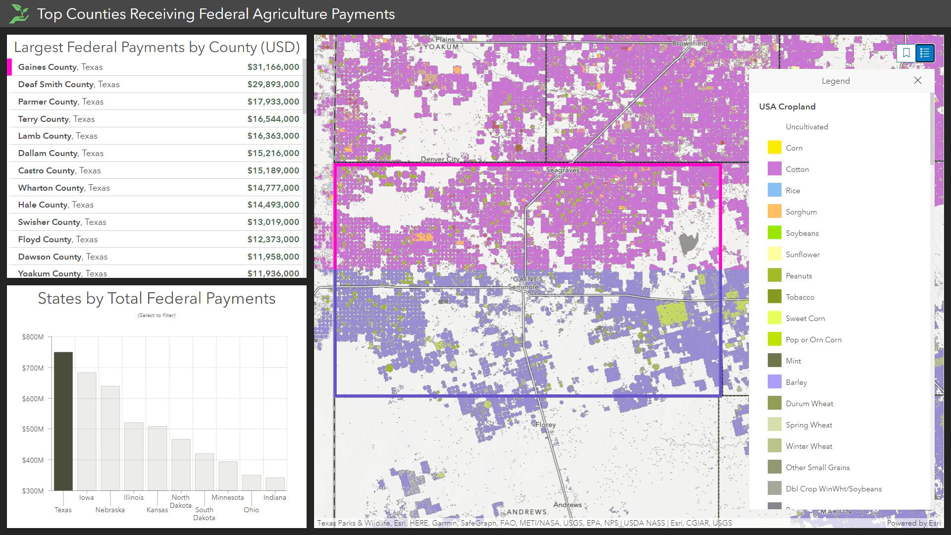
A great way to start exploring the new Census of Agriculture data in Living Atlas is to make an ArcGIS Dashboard. Dashboards are simple to build, easy to use, and provide quick facts about the data using widgets such as charts and ordered lists. This example Dashboard provides simple statistics from the Census Agriculture Federal Payments Layer.
On the left, there is a list widget identifying the counties with the largest federal payments. Selecting a county in the list, zooms to the county on the map so that we can see what crops are grown in that area. For example, the number one county, Gaines County, Texas grows predominantly cotton. According to the chart showing total federal payments by state, Texas is also the state receiving the most federal payments. Charts are also selectable to filter the features shown in the map and county list for further exploration.
To learn more about ArcGIS Dashboards, visit this blog or the documentation. Click here to learn how to make this dashboard.
Use Blending Modes to combine layers
The new blending tools in ArcGIS online and ArcGIS Pro enable you to create a superstar map in minutes. My current favorite blend mode is Destination Atop where you can use one layer to mask another.
For example, we can make a choropleth map of wheat production with layers from Living Atlas. It is a solid map but nothing special:
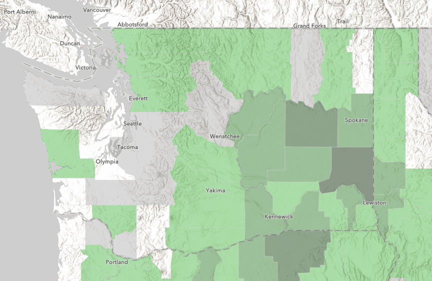
Choropleth map of wheat production in the Pacific Northwest
By simply adding the USA Croplands layer, opening the map in the new Map Viewer, and setting the layer’s blend mode to Destination Atop gives us a much different view of the information:
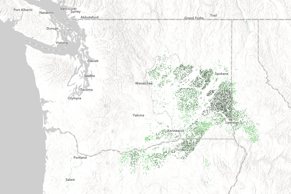
Map of wheat production created from the USDA’s Census of Agriculture county level data masked with the USA Croplands layer
Note how this version of the map better displays the concentration of wheat production in the Columbia Basin of Eastern Washington and surrounding areas in Oregon and Idaho. While small amounts of wheat are grown throughout the region the vast majority is grown in the deep glacial soils and warm, dry summers of the Columbia Basin.
To explore this map open it in the new Map Viewer.
These blog posts are loaded with more ideas on what you can do with blend modes.
Click here to learn how to make this map.
Explore relationships with Smart Mapping
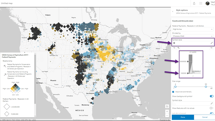
One way to explore new patterns about agriculture is by using the relationship mapping style. A relationship map is a powerful way to compare two different spatial patterns alongside each other within a single map. Instead of making two maps with two distinct patterns, we can overlay these to create a gridded legend which communicates how the two patterns intersect.
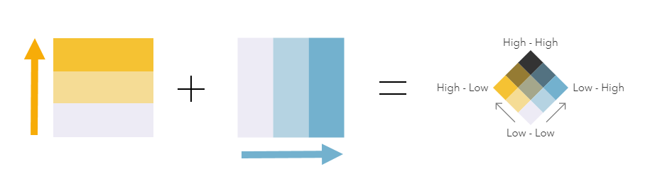
If we take a closer look at the Federal Payments layer from the Agriculture Census, we can learn more about where Federal dollars are being allocated by using this mapping style. For example, this map compares federal payments toward conservation and wetlands versus all other agriculture types. Areas in yellow show where there are above-average amounts of Federal payments toward Conservation in comparison to other types of farming, whereas areas in light blue have a above-average amount of Federal payments toward all other agriculture . Areas in black have an above-average amount of both types of payments. The total amount of Federal payments toward agriculture are emphasized within the map by the size of the symbol.
The key to making this a policy-centric map was the use of national figures to anchor the map. The summary of Federal Government Payments tells us that the average farm got $13,906 in 2017, and the average Conservation/wetlands program got $6,980 in 2017. Using these numbers instead of the default settings helps us learn what is above and below average.
The final web map was then added into the Media Map configurable app to showcase the map in a clean way. To learn more about the relationship mapping style, visit this blog or the documentation for ArcGIS Online.
Click here to learn how to make this map.
Summarize crop types in ArcGIS Pro
Do some crops have more political power than others?
To help answer this question, we calculated the number of cultivated acres for four crops by US Congressional district. We wanted to see if each crop played a role in the local economy of each US Representative.
How did we sum up acres from an image layer by a oddly-shaped geography like congressional districts?
First, we filtered the USA Cropland layer to show only the crop we were interested in, in the most recent crop year. Second, we applied a raster function to recode crops we were interested in to a new integer value of 1. Third, we ran the “Zonal Statistics as Table” geoprocessing tool for each crop to count the number of acres in each district that had a value of 1.
For step by step detail, see the blog “Is Georgia Still the Peach State?” and follow through the steps, almost exactly the same workflow as in this blog.
The USA Cropland living atlas layer is time-enabled so that it may display growing seasons frame by frame as an animation. But we wanted to restrict analysis to only the most current crop year. In ArcGIS Pro table of contents, we applied a filter to make the layer display only the most current crop year, 2019. After that we applied processing templates found in the layer properties to help constrain the layer to a particular crop.
Next we applied a raster function to remap the classes we wanted to a value of 1, and everything else to value nodata. This raster function further filters the USA Cropland layer, simplifying it into a single class for each crop.
Finally we added 117th congressional districts to the map from ArcGIS Online, then for analysis, we chose the geoprocessing tool “zonal statistics as table”. We zoomed the map to the lower 48 states and made this the extent of our analysis, cutting processing time in half. In the environments tab for the tool, specifying a cellsize of 63.615m (the square root of one acre) cuts the analysis time in half again, with the result a table whose count also equals the number of acres. We linked the tables back to the congressional districts using the objectid field (our zone field), added fields for acres by crop, moved the statistics into the fields, and published the layer.
Want to learn more?
- Browse Living Atlas to find content for your GIS workflows
- Connect with us on Esri Community to share your work, ask questions, and learn new things about ArcGIS Living Atlas of the World.
- Find us on Twitter to see what’s new in Living Atlas
- Explore blogs about the newest content added to Living Atlas.
- Explore tutorials within Learn ArcGIS that use Living Atlas content to solve real-world problems.


Article Discussion: