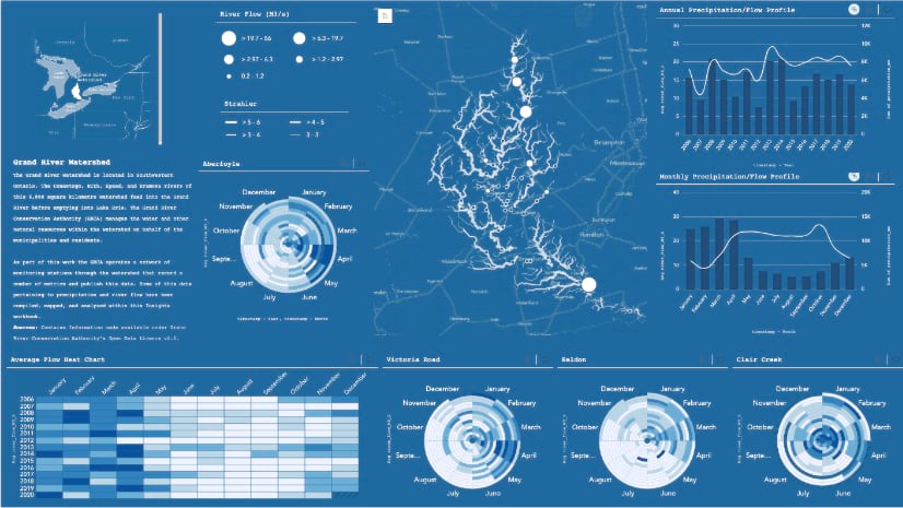
In this series, we’ll be stepping through the workflow for creating an Insights workbook of watershed monitoring data using this map as inspiration. Along the way we’ll be using the analysis strengths of Insights to crank things to ‘11’.
So following along or apply it to your own data analysis project as we set off on creating our next best workbook. Now if only we had some data to plug in and work with…
Thanks to the proliferation of sensors, many datasets are becoming much more readily available. In particular, those datasets pertaining to monitored phenomena are just about everywhere (think earthquakes, weather, and oceans). These datasets are often robust and long running; maintained by scientific, conservation, or government agencies that make the data available for download. However, the harsh reality is that sometimes with great volume, can come great inconvenience:
- Data volume is massive and often split into ‘chunks’ to facilitate transfer.
- Download interfaces put limits on the downloads (temporal ranges, number of sensors)
- Last but definitely not least, field names get changed over the course of the dataset (that’s worth an audible groan).
- [Insert unique personal data complaint here].
Fear not! With a little scripty-business you can piece the data back together, clean it up, and pull it right into Insights!
Still have doubts? Thinking of copy/pasting, removing headers, or collating your data manually? JUST WAIT, I wasn’t sure my scripting skills were up to snuff either but buckle up because we’re going to learn together!
Scripting Groundwork
Pausing just a moment. If scripting in Insights doesn’t ring a bell, get all the background you need from this announcement. It has all the details on the environments supported and how to set everything up. Bonus, it has some samples that are great reference in this GitHub repo (pssst, these proved invaluable for me getting started). Getting your desired environments set up shouldn’t take long, I’ll wait.
All done? Great, now let’s start digging into some data!
Data Collection
The data collection, processing, and analysis for the initial map took longer than I care to admit. Approaching this task with Insights, I was looking forward to letting Insights do the analytical heavy lifting.
I started with gathering the data from Grand River Conservation Authority, my local conservation authority. I was interested in river flow again but many other variables are available from their monitoring datasets. This specific download interface limits the downloads to a 365-day range. However, I was looking to explore the data across a greater date range, I resigned to performing a number of downloads for the stations of interest.
I dumped the files into a ‘Data’ folder for this project to keep things somewhat organized. After I inspected a sample file, I found that the csv has a header with some helpful metadata. Unfortunately, this metadata prevents me from simply smacking the data together. It would also be more useful stored in a column of the dataset since I’m interested in multiple sensors.

Enter a data preparation script, I could author a script to collate the data into a single complete dataset. Furthermore, transposing some of the sensor metadata from the file header into attributes of the dataset would give me a structured dataset containing multiple sensors and additional attributes for later use.

Script
With the data structure in mind, I fired up the scripting environment in Insights and got to work. I dove right into the scripting environment in a new workbook and created a connection to a Python kernel for this project. This is where I’d author the script. You can also, load in previously created scripts, run them with datasets from Insights, and save out any scripts you author as Jupyter Notebook files (.ipynb). For those following along, here’s my completed script for reference.

I started with importing the modules I figured I’d need. In this case, I was going to wade into pandas for the first time. I made thorough use of the developer samples and modelled my script after this snowfall example that performed a similar data assembly.
Gather Datasets
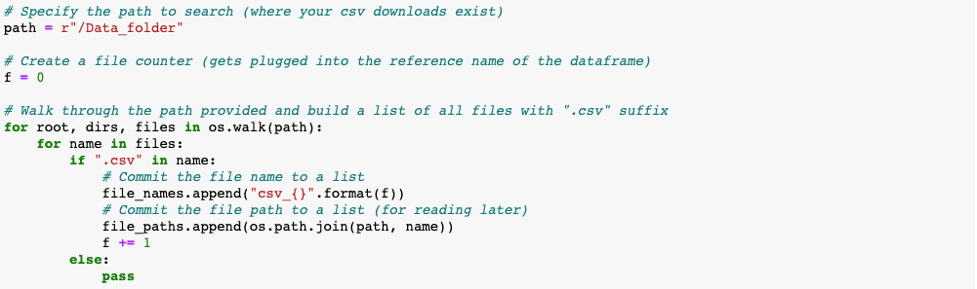
I began by setting my script to walk through my ‘Data’ folder containing my csv downloads and to a list of file names and paths.
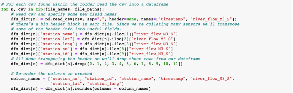
For each of the files collected from my data directory, I’d read those *.csv files into a pandas dataframe. I also transposed some of the attributes from the file header into new fields by referencing their row index within the second column. When complete I dropped these initial rows from the file. Now that my header was removed and I had my new columns, I organized the fields in the file.
Merge and Organize
I concatenated all of the dataframes from the dictionary that was constructed. Moving forward, I’d have a single dataframe to work with in the script.

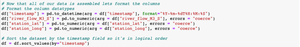
It was at this point I went and added my assembled dataframe to Insights only to realize that I hadn’t specified any datatypes for my fields. Thankfully, I’d saved my script so I could open and modify it to set the column datatypes. I also realized it would be helpful to sort based on the ‘timestamp’ column so all of my data was in order based on when it was recorded.
Inspect Results
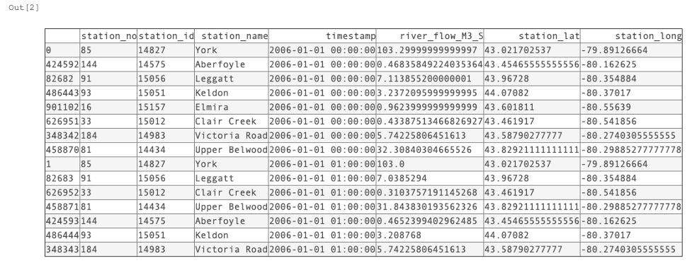
As I authored the script, I regularly used the .shape, .head, and .sample pandas properties to output the results to the Out[ ] cell and reveal how I was successfully, or more frequently unsuccessfully, progressing as I became familiar with pandas. With much more documentation searching and reference to the samples, I ended up with a table with all my data collated and the transposed attributes.
Output Dataset
With that everything I set out to achieve with this dataset was completed. I added the dataframe to the Insights datapane and gave it a descriptive name. I also saved my script as a Jupyter Notebook for safekeeping.

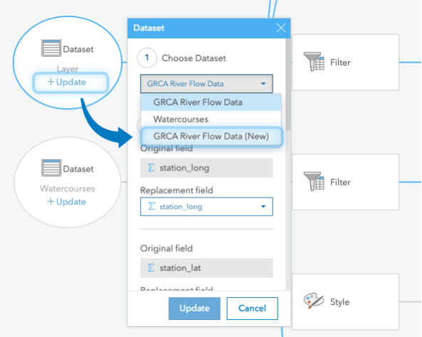
Once saved, this script can be easily re-run with the new results being added directly to Insights. I made frequent use of this as I constantly increased the scope of my dataset, occasionally adding more sensors and further increasing the timeframe. Rerunning my script and then updating the data sources in the Analysis View quickly updated the content of my workbook.
Phew, that wasn’t so bad right? This was just a simple exercise and we managed to collate all of our downloaded datasets into one table, rearrange the fields to improve the structure, and bring the new dataset right into Insights. As you wade deeper into the scripting capabilities, you can further manage and prepare you data and conduct analysis without jumping between applications. The best part is if we need to repeat our analysis, add more data, or modify the scope we can simply run our script again and Insights can refresh our workbook with the new sources (can’t get much more convenient than that, right?).
Stayed tuned for a future walkthrough where we’ll use this dataset to build out a complete workbook with visualizations that reveal trends in the data and eventually create a polished presentation to share with others.


Article Discussion: