In ArcGIS Pro 3.2, three new parameters were added to the arcpy.da.SearchCursors to allow for searching a feature class table by passing in a geometry to this python method. The new spatial_filter parameter is the geometry object by which features are filtered. The spatial_relationship parameter is the relationship between the input query and the query geometry. The default is INTERSECTS, which is what we will use in these tests. The third parameter is search_order, which can be either ATTRIBUTEFIRST or SPATIALFIRST (default). This parameter is only applicable for data hosted in an enterprise geodatabase.
We will analyze the performance of the new spatial filter of arcpy.da.SearchCursor for limiting records by comparing the results of testing with point, line, and polygon input geometries across multiple data sources including a file geodatabase, an enterprise geodatabase, and an ArcGIS Online feature service. To do this we will use three different approaches: the new spatial filter on the Search Cursor, a client-side relationship operation after performing the Search Cursor, and Select By Location before the Search Cursor.
Summary of the data
We will use three different test cases to demonstrate that performance is improved across varying geometries for the input and features to be filtered.
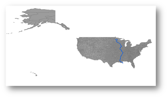
Case 1: US counties that intersect the Mississippi River
Short name: US counties by Mississippi River
Target: US counties, 3,140 polygon features (gray polygons)
Selecting geometry: Mississippi River (blue line)
Number of records selected: 114
Purpose: The selecting feature is quite large in contrast to the entire extent of the data.

Case 2: Select random points that intersect with Italy
Short name: 100k pts by Italy
Target: Random points, 100k points (gray points)
Selecting geometry: Italy (blue polygon)
Number of records selected: 947
Purpose: A large volume of small geometry objects (points) against a single polygon where only 1 percent of the input features get through the filter.
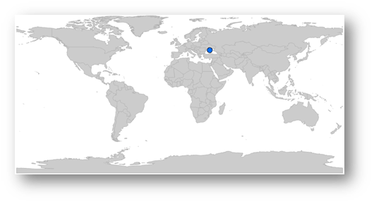
Case 3: Select world countries that intersect a point
Short name: World countries by 1 point
Target: World countries, 248 polygons (gray polygons)
Selecting geometry: A single point (blue point)
Number of records selected: 1
Purpose: The simplest query of searching for what is at a specific location.
Spatial filtering approaches
There are three approaches to filtering and retrieving data that we will contrast in this analysis. The goal for each of them is to retrieve the object ID field (OID) of the spatially filtered subset of the input records.
All three approaches produce the same set of features for each individual case.
Approach name: Cursor with spatial filter
Description: The new parameter to arcpy.da.SearchCursor at ArcGIS Pro 3.2 where filtering is done in the database.
Approach name: Cursor client-side relational operator
Description: Use the regular arcpy.da.SearchCursor, fetching all records and then using the arcpy.Shape.Disjoint() relational operator to select the intersecting records.
Approach name: Select by location
Description: Perform SelectLayerByLocation on the dataset (relationship=INTERSECT), and use arcpy.da.SearchCursor on the layer to retrieve only the selected features.
Note that the layer is created once and that cost is not included in the performance timing.
Results
The following results demonstrate that the new approach with the spatial_filter parameter on arcpy.da.SearchCursor does well in comparison to the other two approaches.
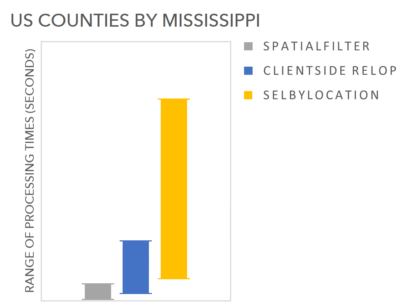
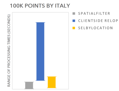
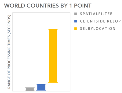
Each chart for the individual test cases contains a bar for each spatial filtering approach that represents the range of processing times in seconds across the three data sources. The bottom of the bar represented the fastest processing time while the top represents the slowest processing time. The approaches are color-coded to gray for the search cursor with spatial filter, blue for the search cursor with the client-side relational operator, and yellow for the select layer by location before the search cursor.
The caveat to these results is that performance will vary with different datasets. Also a variety of factors can affect performance physical hardware, system configuration, network performance and network proximity, database tuning and load. Many of these factors can be particularly impactful for processing remote data sources. The performance times used in the analysis below provide some observed numbers but these comparisons should not be taken as absolute or definitive.
Interpretation of the US counties By Mississippi River test case:
This case is best at showing the performance improvement when using the new parameter to limit larger polygons from being fetched from the data source where they then require being turned into arcpy.Polygon objects for comparison. As you can see in the graph below, the search cursor with the spatial filter performed quicker based on its range of processing times with all three data sources compared to either of the other two approaches. The lower end of the range for the processing times for the client-side relational operator was faster than one of the tests for the spatial filter. However for the same data source it was slower than using the cursor with spatial filter.
Interpretation of the 100k points by Italy test case
The new approach for the cursor with the spatial_filter parameter was the fastest across all tests in this set as well. Even the fastest time for the client-side relational operator was slower than the slowest processing time when using spatial_filter as evidenced by the non-overlapping ranges. Select by location is similar in range in the below chart but if you individually compare by data source then the cursor with spatial filter was faster for all three and has an overall narrower range.
Interpretation of the World countries by 1 point test case
In this test case, you can see that the range of processing times for the cursor with spatial filter is still narrower than the client-side relational operator and faster overall. The ranges for select by location and cursor with spatial filter do not even overlap. This indicates that the slowest processing time for the spatial filter was much faster than the quickest processing time for the select by location.
Conclusion
As demonstrated through this series of tests (27 individual tests overall), the new arcpy.da.SearchCursor spatial_filter parameter performs better than the other approaches for all three types of selecting geometry. Across all three test cases you can notice that the range of processing times is generally much smaller than that of the other approaches, which can vary quite a lot dependent on the data source.
The fact that the spatial_filter approach relied on the database to perform the spatial query and avoids pulling the entire geometry from the database gives it a distinctive performance advantage particularly with remote data sources, but as shown above this new approach performs extremely well with all cases. So with scripts or workflows where performance is a consideration the new spatial_filter parameter may be a good option to evaluate.

Article Discussion: