In an earlier article, I walked through the core trace parameters and framework for the ArcGIS Utility Network. In this article, I will cover a complementary function of network behavior: how attributes can be propagated or substituted through a trace, update, or export operation in the utility network.

Attribute Propagation is a function that is commonly used to represent a variable such as pipe pressure, line voltage or phase.  In either case, there is a condition (pressure, voltage, phase) that is established as a network attribute at a controller and is pushed in the respective direction of the elements of the controlled network.  For example, a pump that establishes a given pressure value can push that value to the connected pipes in the system.  A network attribute is defined to not only persist the pressure value in the controller but also for other features in the subnetwork.  A second network attribute is configured to enable the user to update or change the propagated network attribute at the device level and have that updated value propagated downstream.

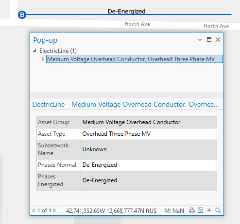
You might ask what’s the difference is between attribute propagation and a field calculation or other functions.  Field calculations are a traditional operation typical of database applications, but attribute propagation takes advantage of the network topology in its native binary form.  For example, let’s create a simple subnetwork with a Circuit Breaker, Transformer, and a Medium Voltage Overhead Conductor. By default, the Phases Energized field is set to De-Energized; this field is populated when you run Update Subnetwork.

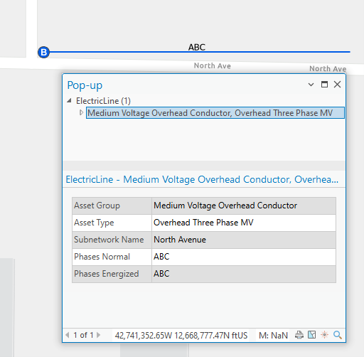
To run an update subnetwork operation, you must first enable the Circuit Breaker as a subnetwork controller for the subnetwork. After doing this and running Update Subnetwork, you can see that the Subnetwork Name and Phases Energized attribute fields are populated. The below graphic shows that the features now belong to the North Avenue subnetwork and the Normal Phases attribute value (ABC) from the Circuit Breaker has been propagated to set the Phases Energized field value on the line.

This is a very simple example of how propagation works.  There are three types of Functions that enable propagation and substitution for the utility network; they are Propagated_MIN, Propagated_MAX, and Propagated_BITWISE_AND.

Propagation Functions

Propagated_MIN which sets a propagated value based upon the minimum value encountered.  An addendum to the Propagated_MIN can be set with a greater or less than value.  Using a downstream trace on an electric network where MOV represents a Network Attribute MOV which is assigned to a given field (https://pro.arcgis.com/en/pro-app/latest/help/data/utility-network/network-attributes.htm).  An example of using the Propagated_MIN function could be found in networks where multiple voltage states might exist in a single tier.   The example below uses a function: MOV PROPAGATED_MIN IS_GREATER_THAN 15 MAXVOLTAGE.

The trace begins with a MOV attribute on each edge and junction element.  The first MOV value at the controller is set as the initial propagated value until the 25kV value is reached, which changes the propagated value to 25kV.  The 25kV value is continued regardless of higher MOV values until it reached the device set at 15kV which is established as a de-energized state in the context of the function operator and sets the propagated value at 0.

Propagated_MAX sets a propagated value based upon the maximum value encountered.  An addendum to the Propagated_MAX can be set with a greater or less than value in a manner like that shown in the previous example.   Next, you will explore the function: MOV PROPAGATED_MAX IS_LESS_THAN_OR_EQUAL_TO 30 MAXVOLTAGE.

This downstream configuration directs the system to continue to propagate the highest value if MOV remains less than 30kV.  The location where 35kV exists acts as a barrier and returns de-energized values for the remaining features.

Propagating conductor phase values requires a bit of a different approach.  The Propagated_BITWISE_AND function utilizes a bitset that represents the various conductor phase configurations are represented as three bits together with 8 for Phase N (neutral), 4 for phase A, 2 for phase B, and 1 for phase C; a state where ABCN is displayed it would be represented as the value 15.  If only AB is configured, that value would be 6, but you can change the bit values and description when you set the coded domain values of the network attribute.

You can use a downstream trace to show how phase propagation can be configured to update phase configurations based upon Phases Current PROPAGATED_BITWISE_AND INCLUDES_ANY ABC PHASEENG (where ABC PHASEENG = 15).  This indicates that the traversal will continue while any phase is in an energized state along the lines.

In this example PHASEENG (Phases Energized) is the attribute updated by the update subnetwork operation. The device with a Phases Current value of  AC restricts the propagated value, while the final device with a Phases Current value of B cannot be energized by the propagated value which causes it to become de-energized.

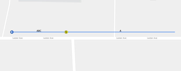
You can see an example of this below. By placing a single-phase switch on a three-phase line you can see that it restricts the phasing on the main line and the tap line it is connected to..

Propagation and Attribute Substitution are configured as part of the subnetwork definition for a Tier in the utility network. Note that the subnetwork definition can only be changed when the utility network is in a disabled state. As shown in the image below, when setting the Propagators parameter using the Set Subnetwork Definition tool, a network attribute is defined on the field to store the propagated value (Propagated Attribute) and a separate network attribute is set as the defining field (Attribute).  A third network attribute can also be defined for setting values for substitution (Substitution Attribute). The Function value establishes the type of function used (MIN, MAX, Bitwise_AND), the Operator value indicates the specific condition that is used during the execution of the query, and the Value represents the binary value that is compared with the calculated propagated value during each trace operation.

Attribute Substitution

Going back to the earlier subnetwork you can see the effect of attribute substitution at a new tap point.  The new line segment that pulls up from the tap point (purple) is configured to substitute the A phase of the line with a phase value of B. This means that when phasing is propagated to the tap line the phase value of A will become B. You can see the effects of this in the screenshot below.

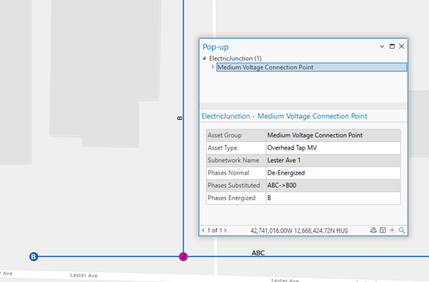
The first thing to notice is that the tap line displays an energized phase of B, even though there isn’t a B phase on the upstream line. The second thing worth noticing is that the phasing or the main line downstream of the tap remains unaffected.

An important consideration to remember with attribute substitution is that it is a diminishing function and does not allow for additive functions. As an example, a single energized phase can transition to another single energized phase, but it cannot transition to two energized phases.

The ability to set these advanced configurations enables utilities to model wire and pipe operational behaviors based upon load or pressure values. Network propagation and substitution are functions designed to provide better experiences for ArcGIS Utility Network users.  These capabilities are used to represent the properties of pipe or wire networks and the engineering properties of the respective configurations.  As the network platform continues to evolve these capabilities will continue to grow and adapt to the needs of utilities and facilities managers.

Conclusion

If you’re interested to learn more about tracing and analysis with ArcGIS Utility Network, you should visit the Analysis and Tracing with ArcGIS Utility Network learning series. This series contains a collection of articles, videos, and tutorials to help familiarize you with tracing, subnetworks, and ArcGIS Utility Network. You can also find more some practical industry-specific examples in the Propagation and Electrical phasing article on the Esri Community site.

If you have specific questions about how to solve different workflows, please visit us on the ArcGIS Utility Network channel on the Esri Community site. This is an active community with thousands of active members.