The intersection of machine learning and GIS is getting broader as we ask increasingly pragmatic questions related to complex spatial phenomena. Whether it is predicting traffic patterns in L.A. or the probability of being hit by the next big storm, we need answers to critical questions to make impactful decisions.
In this blog, we’ll explore an essential component needed towards answering such a question: what will the future climate be in U.S.? This question requires calibrating a global climate model with spatially-limited local temperature measurements. In a planet that is constantly warming, calibrating global climate models is vital to answer questions ranging from what will the average temperature be in Redlands in November 2050 to which Canadian cities will be wine country in the future.
For climate models, calibration can be done using regression methods and we will explore the use of different types of machine learning methods for regression. Here, we break these methods into three different types depending on whether spatial consideration is a part of the method itself or not. From an analysis perspective we will explore the 3 different approaches to solving a spatial prediction problem:
- Non-spatial (generic) machine learning
- Spatial machine learning
- Non-spatial machine learning with geoenriched predictors
Predicting Weather: Need for Climate Downscaling
Scientists use Global Climate Models (GCMs) to model mesoscale to large scale (100s of kms) atmospheric dynamics of our planet. GCMs solve analytical equations, such as Navier-Stokes equations, to model global air flow and energy transfer in the atmosphere. In addition to global dynamics, weather is impacted by local effects such as distance to a water body, proximity to mountains, etc. These local effects are not modeled in GCMs. Thus, GCMs need to be calibrated with measurements collected at a finer scale. Fine scale measurements of weather such as local temperature comes from weather stations that collect data continuously. In this analysis, we will be using weather measurements from a subset of weather stations in U.S. and CGCM1 climate model. Both of the data sources are below, weather stations are symbolized with black points and GCM grid over U.S. in red:
Predicting future temperature using a GCM requires forming a statistically-valid relationship between coarse-scale climate model and fine-scale weather measurements using observed data. We will use 19 variables from CGCM1:
- Mean sea level pressure
- Airflow strength (simulated at 3 pressure levels)
- Surface zonal velocity (simulated at 3 pressure levels)
- Meridional velocity (simulated at 3 pressure levels)
- Surface vorticity (simulated at 3 pressure levels)
- Geopotential height (simulated 2 pressure levels)
- Zonal velocity (simulated at 2 pressure levels)
- Near surface relative humidity
- Near surface specific humidity.
We will establish a relationship between simulated climate variables and measured average temperature to calibrate GCM. This process is known as downscaling and it can be done a number of ways (Wilby and Wigley, 1997). In this blog we will explore statistical downscaling. For the sake of demonstration, we will downscale GCM variables for the time-snapshot 12th of March 2012 for contiguous U.S.
Climate Downscaling Using Generic Machine Learning Methods
Machine learning methods, in this case regression methods, that are not crafted towards a specific type of feature such as spatial features, provide a general relationship between predictors (GCM variables) and the target variable (average temperature). We will utilize Support Vector Machine (SVM) and Ridge Regression methods from Python’s scikit-learn library to define a predictive model. The reason behind this choice is the ability of both methods to model non-linear and complex relationships.
One consideration for these methods is over-fitting. For temperature profile prediction, it implies forming a regression model that predicts temperature accurately at weather station locations but that cannot produce accurate results else where. Regularization parameter for Ridge Regression controls over-fitting directly and for SVM it is finding a combination of parameters that avoid over-fitting which can be a time-consuming process. We wrapped SVM and Ridge Regression into a Python toolbox so that we could consume scikit-learn functionality as a geoprocessing tool in ArcGIS Pro. You can reach the Python toolbox used for this project here. The toolbox has the benefit of making the functionality easily shared with other ArcGIS users who may not be as familiar with scikit-learn and observing the impact of model parameters on the predicted average temperature profile.
Predicted average temperature using 19 GCM variables are plotted against observed average temperature below:
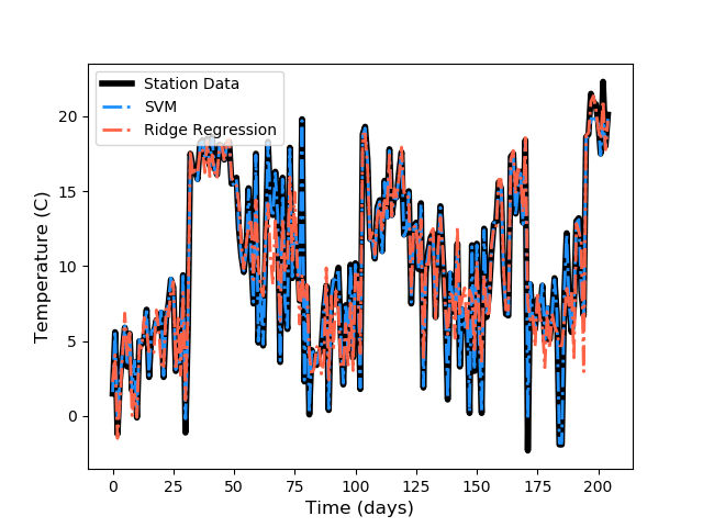
Figures above show that Ridge Regression does not predict average temperature at weather stations as accurately as Support Vector Machine. For a spatial problem such as predicting temperature over contiguous United States, we also need to map the results to investigate if we can capture overall patterns in spatial temperature variation.
Mapping the results for a spatial prediction makes over-fitting apparent for SVM. Although SVM can predict average temperature almost perfectly at weather station locations, it fails to produce sensible results else where and produces a patchy temperature profile. On the other hand, Ridge Regression can generalize the prediction with an optimized regularization parameter, however the value for this parameter has no spatial meaning for temperature downscaling.
Incorporating “The Where” at the Algorithm Level: Spatial Machine Learning
Previous methods are non-spatial methods that do not incorporate spatial information in the context of downscaling. Temperature profiles show spatial patterns, thus it is safe to define downscaling and temperature forecasting as a spatial problem. Next, we performed downscaling using spatial regression methods from ArcGIS Pro. These methods are formulated to model spatial relationships implicitly in their formulation.
One these methods is Geographically Weighted Regression (GWR) that defines the downscaling with a spatially-varying linear regression. At any prediction location, GCM values from nearby neighbors will drive the predicted average temperature value with locations further away having less impact on the regression. Secondly, EBK Regression Prediction was used to form a relationship between observed average temperature and the simulated variables of GCM. EBK Regression Prediction creates subsets of the data and models the spatial relationships using two-point statistics, in particular semi-variograms.
Simply put, both of these methods put Tobler’s law in action by forming relationships between spatial objects that are close in space. GWR requires the predictor variables to be independent. After a simple analysis of correlation coefficients between 19 GCM variables 3 that were seemingly independent were used: specific humidity at 850 hPa, vorticity at 850 hPa and surface zonal velocity. Note that EBK Regression Prediction does not have this limitation but we performed spatial regression with 3 predictors instead of 19 to show the power of space in analysis.
Both methods create a temperature profile that shows expected spatial patterns of temperature and fit observed temperature values at weather stations. These methods differ than generic machine learning methods in that they need spatial data to define relationships between predictors and the target variable. Incorporating space results in means that we get reasonable results, without the patchy, overfit appearance of the non-spatial methods, and we only needed 3 variables to do it.
Incorporating “The Where” Using Geoenrichment: Forest-based Prediction in ArcGIS Pro
Tree-based regression methods have been popular due to their flexibility in types of predictors and target variables they can handle, small number of assumptions in their definition and their ability to capture complex relationships in data. We explored using a forest-based prediction implementation from scikit-learn to answer a spatial classification problem in a previous blog. Similar to SVM and Ridge Regression, forest-based prediction has no concept of space in its definition, however spatial feature engineering, also know as geoenrichment, allow including spatial information in forest-based regression. We will explore the impact of including a spatial predictor using forest-based prediction.
Large water bodies such as seas, lakes and oceans impact the local temperature. We represent this domain knowledge using a spatial variable, distance to water bodies. We will use the new ArcGIS Pro implementation of a forest-based prediction that allows incorporating different sources of spatial data such as distance features, rasters and vector data. Below, we compare two predictions: one uses 19 GCM variables as predictors and the other uses the same 19 variables and a distance to water body raster.
Forest-based regression on the left explains small scale temperature variations due to proximity to water bodies. Thus, including a spatial predictor in a non-spatial regression method still allows capturing some complexity pertaining to a spatial phenomena. It is interesting to note that geoenriched predictor shows some similarities to the EBK Regression Prediction result. In Pacific and Mountain regions of U.S. both methods find two distinct regions of low temperatures, whereas forest-based regression model using simulated GCM variables only find three distinct low temperature regions (one in Pacific region).
What’s next? Forest-based Prediction and Updated GWR
Different approaches to statistical downscaling reveal how different machine learning methods can be used to solve an inherently spatial problem such as estimating a temperature profile. Generic machine learning methods are general in the types of problems they can solve but for spatial problems they require representation of spatial relationships. Ridge Regression from scikit-learn eventually produced a reasonable result without geoenriched predictors. However, values for tweaking parameters that produce a feasible temperature prediction does not lead to understanding the spatial phenomena.
Both GWR and EBK Regression Prediction created reasonable average temperature profiles without non-spatial tweaking variables and by using only one-sixth of the inputs used for Ridge Regression and SVM. Thus, parsimonious models are created with spatial regression models that incorporate spatial relationships into regression implicitly.
Lastly, the value of spatial feature engineering is demonstrated using a distance feature with GCM variables to predict average temperature using a forest-based predictor. Distance to water bodies was one of the top 10 most important variables (as per the forest model) among 19 GCM variables.
We are devoted to grow the ArcGIS platform in the area of machine learning to answer critical questions pertaining to complex systems with data-driven methods. Thus, in one of the new tools in Pro 2.2 will be ESRI’s take on forest-based prediction, an algorithm although non-spatial in its design allows you to incorporate space into your analysis so that you can make predictions and classifications using geoenriched variables. In the Pro 2.3 timeline, we will be updating one of our spatial regression methods, GWR, so that it has broad applicability in terms of types of predictions it can make: Geographically-Weighted Logistic and Poisson Regression to name a few.

Commenting is not enabled for this article.