In this three (or more) part blog series, I present examples of workflows in ArcGIS Pro to explore the many dimensions of environmental security. These blogs don’t contain detailed step-by-step instructions but should provide sufficient detail for you to reproduce each analysis and explore on your own.
When most people think about national security threats, they envision invading armies or hackers stealing intellectual property. However, while these traditional threats to national security still exist, the long-term impacts of climate change arguably present a more ubiquitous and persistent threat. Rising sea levels, more frequent and severe drought, and extreme heat events drive mass migration, increase food insecurity, stress critical infrastructure, and induce social and political unrest.
Climate change: the primary driver
In strong language rarely used in the scientific community, a recent report by the Intergovernmental Panel on Climate Change (IPCC) stated that “it is unequivocal that human influence has warmed the atmosphere, ocean and land. Widespread and rapid changes in the atmosphere, ocean, cryosphere and biosphere have occurred.” Human-caused changes to our planet are the primary drivers of the events and trends that impact our security.
GIS has been at the forefront of assessing potential climate impacts and developing and prioritizing mitigation strategies. The GIS for Climate Hub shows many excellent examples of these efforts. GIS-based climate workflows often focus on identifying patterns — the what or where question. In this blog, we’ll focus more on a when question – can we identify changes to the seasonal patterns of weather events.
Generally, when does the warmest day of the year occur?
Intuitively, the warmest day of the year should occur in the northern hemisphere on June 21 (summer solstice), when the amount of solar radiation received is at its maximum. However, large-scale (synoptic) weather patterns can impact when the warmest day occurs at different locations. To establish a baseline for the warmest day, we can explore modeled temperature data. The NARR model contains daily temperature data from 1979 through 2020 and is available in netCDF format. However, each year comes in a separate file (air.sfc.1979.nc, air.sfc.1980.nc …). To combine the data into a single dataset, I created a multidimensional mosaic dataset using the Create a mosaic dataset from netCDF files workflow.
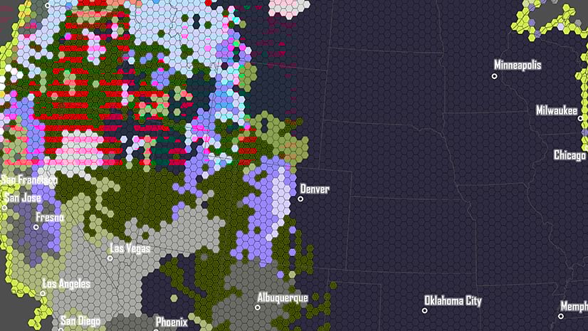
The resulting mosaic dataset contains 15,341 slices representing the daily average temperature for each 32 square kilometer pixel in north America. Next, I used the Aggregate Multidimensional Raster tool with the recurring daily keyword to produce the average daily temperature for each day of the year. The recurring daily keyword causes the tool to aggregate multiple years of daily data into daily time steps where the result includes one aggregated value per Julian day. The output includes, at most, 366 daily time slices. Finally, I used the Find Argument Statistics tool with the argument of the maximum statistics type to find the Julian day of the highest temperature. After clipping the result to the conterminous U.S., here is the result.
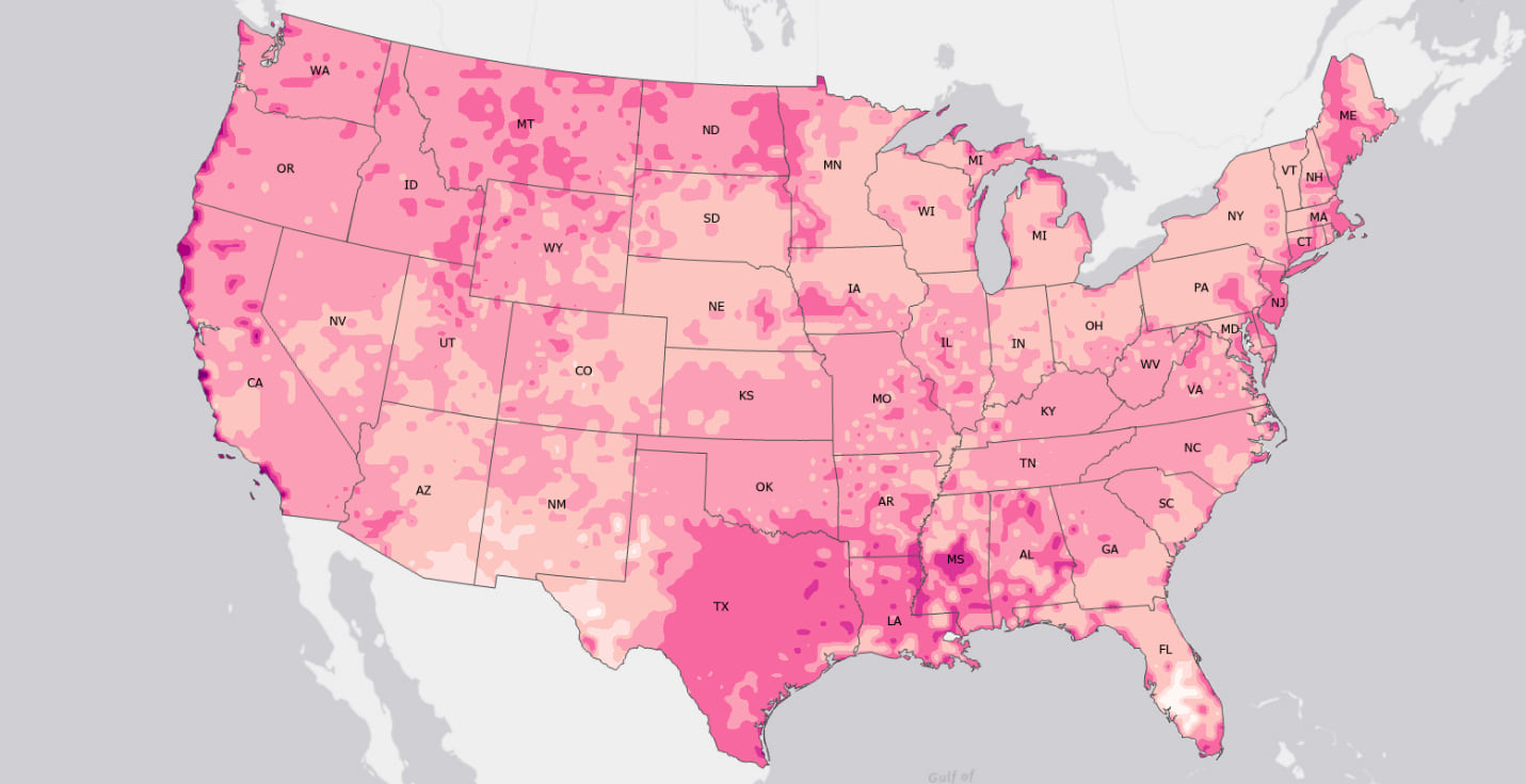
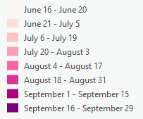
This map approximates the National Centers for Environmental Information (NCEI) Warmest Day of the Year maps, and they provide explanations for similar patterns. For example, the warmest day occurs earlier in Arizona and New Mexico than in the rest of the southwest because of the North American Monsoon. Mid-summer monsoonal clouds and rain reduce temperatures in these areas. In addition, the coastal marine layer along the west coast delays the onset of warmer weather. Can you identify other patterns?
Is the warmest day of the year occurring earlier or later?
The previous example used modeled climate data to establish a baseline of when to expect the warmest day of the year. However, similar methods can analyze observed meteorological data. For example, the Global Historical Climatology Network (GHCN) archives daily climate summaries across the globe. We can use these datasets to explore whether the warmest day of the year is occurring earlier, later, or not changing. However, meteorological data are inherently messy – instruments malfunction, transcription errors occur, and weather stations are regularly commissioned and decommissioned. As a result, weather data always requires careful validation and cleaning – a task we refer to as data engineering. Using the new Data Engineering capabilities in ArcGIS Pro, I cleaned the tens of millions of GHCN records and identified 3,572 stations in the conterminous U.S. that had consistent observations from 1991 through 2020. Then, using the Create Space Time Cube From Defined Locations tool, I created a space-time cube to explore how the Julian day of the warmest day of the year is changing across time at each station. When the space-time cube is created, a Mann-Kendall trend test is calculated for each station to determine whether the Julian day of the warmest day is occurring later, earlier, or not significantly different. The following map summarizes the trend for each station.
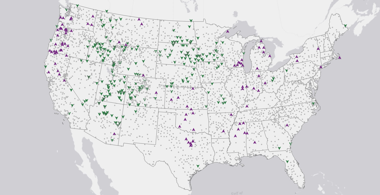
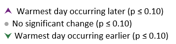
Fascinating patterns emerge. There are two areas, the Pacific NW/Northern California and the central southern states, where we see statistical evidence (p ≤ 0.10) that the warmest day is occurring later in the year. The majority of the stations in the Pacific NW are in a historically temperate, dry, and warm summer climate regime (Koppen-Geiger Csb classification based on visual comparison to updated maps produced by Beck et al. 2018). The stations in the southwest are in a temperate, no dry season, hot summer climate regime (Beck 2018 category Cfa). Global increases in temperature and the resulting increases in summer storms likely delay the onset of warm summer temperatures in these areas.
Stations in two areas, the western Great Plains and the Upper Midwest are experiencing their warmest day earlier. However, here the patterns are contrasting. The stations in the western Great Plains are in an arid, steppe, cold climate (Bsk), while the stations in the Upper Midwest are cold, with no dry season, and have hot summers (Cfa).
Implications for environmental security
The analyses conducted for this blog suggest that summer temperature patterns are changing. A growing body of research supports measurable disruptions to seasonal patterns of temperature and precipitation. For example, Jiamin Wang and colleagues have shown that summer has increased from 78 to 95 days between 1952 – 2011 in the northern mid-latitudes (Wang et al., 2021). Disruption to seasonal patterns can have profound effects related to environmental security:
- Energy security – extended summers place additional strain on outdated and often overtaxed power distribution systems. For example, in February 2021, millions of Texans were without power for several days due to a series of severe anomalous winter storms. Reliable, sustainable, and affordable energy is critical to economic health and growth. In addition, increased energy demand potentially increases dependence on imported energy. Six stations in western Texas have their warmest day occurring later, portending increased demand on an isolated power distribution system. In addition, Texas houses 19 military installations, most located in western Texas.
- Food security – Researchers have identified that the “two most prevalent drivers of altered crop yields are changes in pollination and pest infestation” (Stevenson et al., 2015). Specifically, milder winters and extended growing seasons allow earlier and longer migrations of crop-destroying pests such as winged aphids. According to the U.S. Department of Agriculture, “Oregon, Washington, and Idaho together are the #1 producer of 22 key agricultural commodities.” Of some concern, all three of these states have statistically significant changes in when their warmest day occurs.
- Physical/border security – Climate change-induced natural disasters such as floods and hurricanes can drive mass migration, straining infrastructure and leading to social and political unrest.
Ideas for the next step
- Replicability and reproducibility are fundamental to good science. You are encouraged to repeat the analyses outlined in this blog with other data sets to see if you get similar results or answer additional questions. Consider using the excellent global data set of gridded daily temperatures (HadGHCND) if you want to avoid the lengthy but necessary data engineering step.
- Climate change is not only impacting when the warmest temperature occurs but also when the coolest day occurs. Explore the methods outlined in this blog to identify when the coolest day of the year occurs.
- While extreme events (warmest and coolest days) are interesting, sustained time periods of high and low temperatures also impact environmental security. The Find Argument Statistics tool can also identify the duration of meteorological conditions. For example, what was the longest period when the temperature was above 90 degrees?
- Look for additional blogs in this series.
References
- Beck, H.E., N.E. Zimmermann, T.R. McVicar, N. Vergopolan, A. Berg, E.F. Wood: Present and future Köppen-Geiger climate classification maps at 1-km resolution, Nature Scientific Data, 2018.
- IPCC, 2021: Summary for Policymakers. In: Climate Change 2021: The Physical Science Basis. Contribution of Working Group I to the Sixth Assessment Report of the Intergovernmental Panel on Climate Change [Masson-Delmotte, V., P. Zhai, A. Pirani, S. L. Connors, C. Péan, S. Berger, N. Caud, Y. Chen, L. Goldfarb, M. I. Gomis, M. Huang, K. Leitzell, E. Lonnoy, J.B.R. Matthews, T. K. Maycock, T. Waterfield, O. Yelekçi, R. Yu and B. Zhou (eds.)]. Cambridge University Press. In Press.
- Lanicci, J. M., Murray, E. H., & Ramsay, J. D. (2019). Environmental security: Concepts, challenges, and case studies. American Meteorological Society.
- Stevenson, T. J., Visser, M. E., Arnold, W., Barrett, P., Biello, S., Dawson, A., … & Helm, B. (2015). Disrupted seasonal biology impacts health, food security and ecosystems. Proceedings of the Royal Society B: Biological Sciences, 282(1817), 20151453.
- Wang, J., Guan, Y., Wu, L., Guan, X., Cai, W., Huang, J., et al. (2021). Changing lengths of the four seasons by global warming. Geophysical Research Letters, 48, e2020GL091753. https://doi.org/10.1029/2020GL091753Received 17 NOV 2020Accepted 10 FEB 202110.1029/2020GL091753


Good day,
Thank you for the great post. In paragraph 8 of the blog, it is mentioned that “when the space-time
cube is created, a Mann-Kendall trend test is calculated for each station, to determine whether the Julian day of the warmest day is occurring later……”
Can you kindly elaborate on how do you then determine whether the Julian day of the warmest day is occurring later, earlier, or not significantly different from the space time cube in Pro – what are the steps?
Do you need to first mark the hot julian day in the space-time cube identified in the blog’s first section? Do you then use generate trend raster? Kindly share the steps for clarity.
Thank you