The ArcGIS Pro 2.2 release has an exciting new machine learning tool that can help make predictions. It’s called Forest-based Classification and Regression, and it lets analysts effectively design, test, and deploy predictive models.
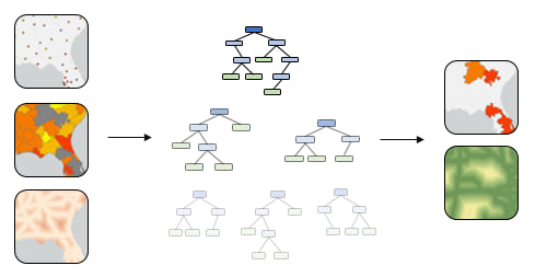
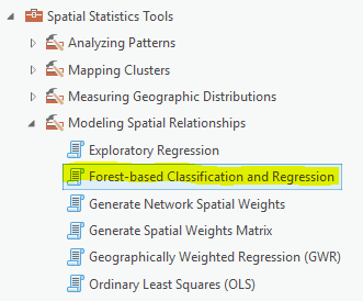
Forest-based Classification and Regression applies Leo Breiman’s random forest algorithm, a popular supervised machine learning method used in classification and prediction. The tool allows analysts to easily incorporate tabular attributes, distance-based features, and explanatory rasters to build predictive models and expands predictive modeling to become accessible and possible for all GIS users.
To show off what’s possible with Forest-based Classification and Regression, we tackled a popular problem in the data science community: predicting home sale values. Let’s take a look at a basic exercise to build a model that incorporates spatial factors to help improve the prediction of home sale prices in California.
Predicting House Prices in California
We’ll start by using the popular California Housing Dataset from Kaggle, containing tracts in California with a series of aggregate attributes for the homes in each tract.
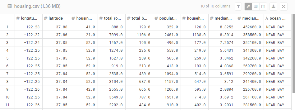
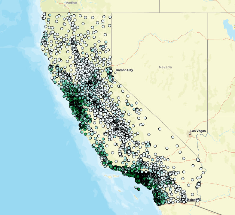
It’s tough to do anything meaningful just by looking at the above table, so let’s make a map of each tract, symbolized by average home sale value at each location:
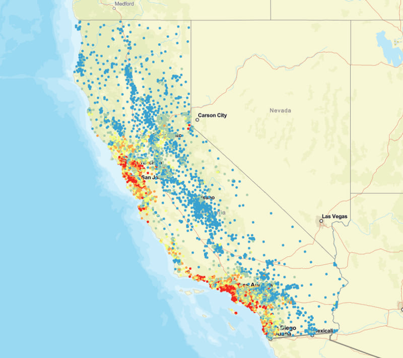
In this map, each point signifies the centroid of a tract in California. The color range represents the average home sale value of all homes in the tract. Blue represents low sales values, yellow represents medium sales value, and red represents the highest values.
Just from viewing this map, do you notice any general pattern?
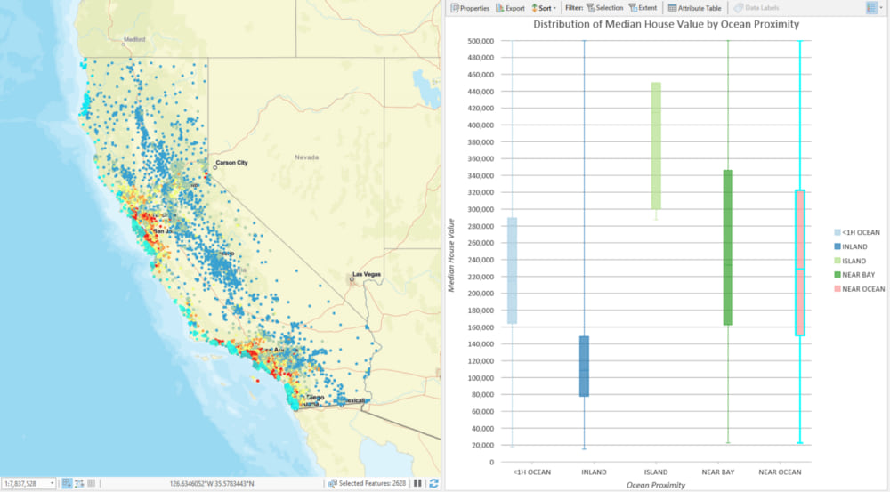
You may notice that higher-priced homes are situated near the largest metropolitan areas. You may also notice that higher-priced homes are situated near the coastline. A quick exploratory chart in ArcGIS Pro helps us explore these patterns:
Let’s view the rest of the data in the provided table. Each record contains a few basic data points for all the homes in the tract:
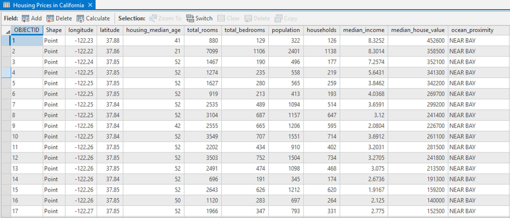
The median house value for each tract is our variable to predict, and these attributes are likely important in helping estimate each value.
We’ll start by following the example provided by Aurélien Geron in his book Hands-On Machine Learning with Scikit-Learn and TensorFlow, where a random forest model was built using primarily non-spatial factors (i.e. the attributes in the table shown above). We’ll compare this model to a second model where we start to bring in other GIS layers to assess how each tract’s proximity to locations of interest may help the model improve when estimating median house values.
Non-spatial Model
Our first model will follow the lead of the Hands-On Machine Learning with Scikit-Learn and TensorFlow example, using the following characteristics for each tract record:
- Median Income
- Housing Median Age
- Total Rooms
- Total Bedrooms
- Population
- Households
- Ocean Proximity
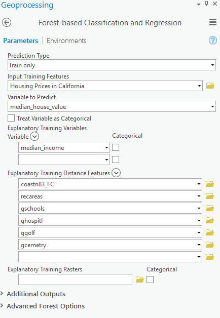
Let’s open the Forest-based Classification and Regression tool and get started:
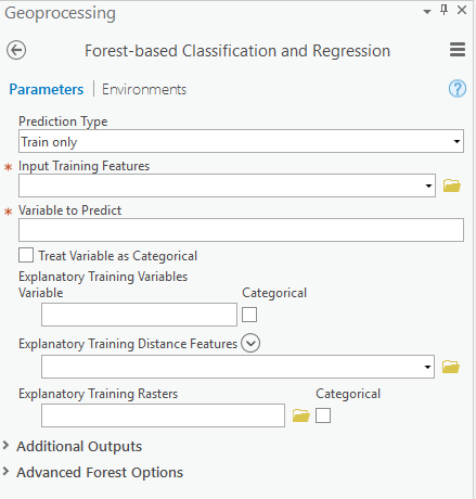
The first parameter designates the type of run you want to execute. For this basic exploration we want to assess model diagnostics (i.e. predictive performance) and monitor changes as we introduce and test combinations of factors. For this reason, let’s leave this parameter at “Train only”.
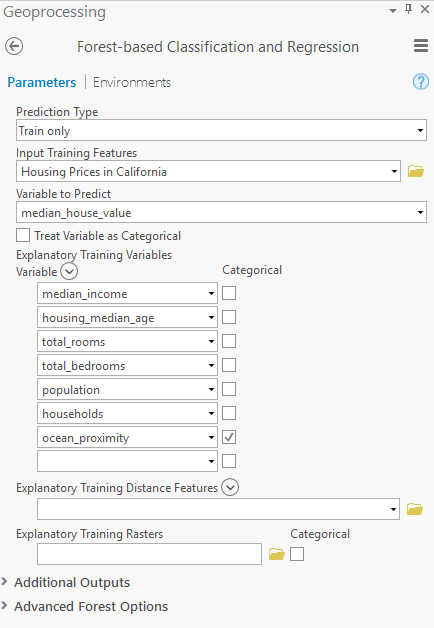
We will specify the input training features, passing our GIS layer of tracts in California, our variable to predict, using the “median_house_value” attribute, and then specify which attributes will be used for the model in the “Explanatory Training Variables” parameter section by selecting each corresponding column in your input data. When complete, your geoprocessing tool inputs should look like this:
Once you execute the model, the tool builds a forest that establishes a relationship between explanatory variables and the designated variable to predict. For more information on how this tool works, please be sure to read this.
Once the tool finishes its run, you should receive a detailed diagnostic of your model performance:
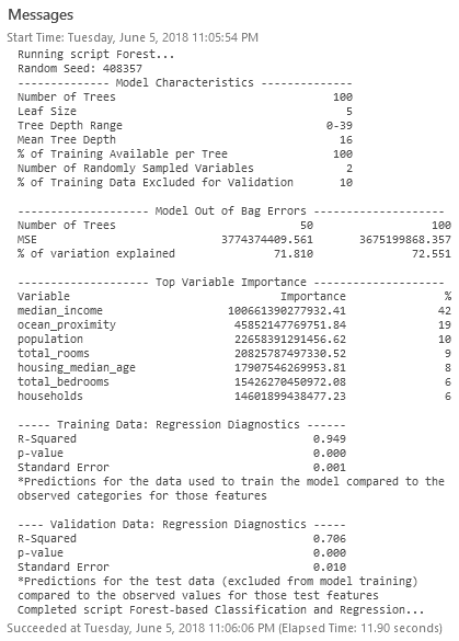
The assessment of top variable importance provides a general sense of which factors helped the model (median income and ocean proximity mattered a great deal). For now, let’s make note of our R-Squared value: 0.706 (this may differ slightly when you execute).
Please note: To create a model that does not change in every run, a seed can be set in the Random Number Generator environment setting. There will still be randomness in the model, but that randomness will be consistent between runs.
Spatial Model
Now that we tried the original approach of estimating home sale values that primarily uses non-spatial factors, let’s explore how the model changes as we introduce distance-based training features. The goal is to compute the distances between each tract and a series of potentially important features that relate to home prices. For our simple exploratory exercise, we’ve brought point feature classes of golf courses, schools, hospitals, recreational areas, and cemeteries. We will also bring in a polyline feature class of the California coastline.
To calculate all those distances, you could conceive of a script to iterate on each record and run some proximity functions to determine the distances between each geometry record… or you could simply open the Forest-based Classification and Regression tool and drag and drop each feature class into the Explanatory Training Distance Features parameter:

Once you have each distance feature loaded, we can run the tool. Our parameters at this point looked like this:
Feel free to experiment with your own potential explanatory training factors! A brief example: Can you find a dataset of public transit station locations, bring it into your ArcGIS Pro Project, and load the locations to the Explanatory Training Distance Features parameter? How does this factor change your model?
Once the tool runs, we can evaluate our diagnostics and compare with the original model:
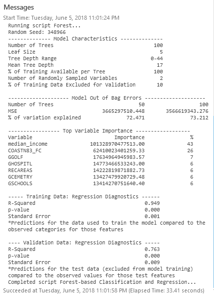
The new regression diagnostics land at an R-Squared of 0.763. Interestingly, a basic model with mostly distance-based factors performed a bit better than the original model that mostly considered the non-spatial characteristics of the homes (number of bathrooms, etc.). If anything — this is data-driven proof of the location, location, location adage!
The run of the tool will also provide the model outputs across your input data:
This isn’t inherently useful on its own since we are basically predicting on records with known values, but it’s useful to see how distance-based features change the model performance. Better yet, its extremely useful to be able to incorporate existing additional GIS data into the model’s considerations for proximity in such a fast and intuitive way.
Note: An additional important aspect of Forest-based Classification and Regression is the way in which the effects of multicollinearity in candidate explanatory factors does not prevent you creating effective models. To understand how random forest mitigates for issues with multicollinearity, I encourage you to explore further in the tool documentation and in additional random forest documentation.
Conclusion and Resources
Performing analysis to predict any event or value is sure to be an exploratory, iterative, messy, and time-consuming exercise. To support these workflows, we need tools that help us quickly incorporate spatial data, support testing, let us quickly evaluate results, and allow us to repeat until we reach a satisfactory result.
Forest-based Classification and Regression extends the utility of the powerful random forests machine learning algorithm by incorporating the ability to consider not just attribute data in your models, but also distance-based training features and explanatory rasters to leverage location in your analysis.

Resources
Forest-based Classification and Regression Tool Documentation
How Forest-based Classification and Regression Works
Use of Forest-based Classification and Regression in Asthma Hospitalization Case Prediction


Commenting is not enabled for this article.