Real-Time Change Detection with Arcade Track Functions in ArcGIS Velocity

Introduction

In this blog, we explore how to use Arcade Track Functions in ArcGIS Velocity to perform change detection. We will focus on monitoring stream gauges with the goal of assessing if water levels are increasing, decreasing, or have not changed since the last observation.

In many situations, the Detect Incidents tool, available in real-time and big data analytics in Velocity, can open and close incidents when certain conditions exist in a continuous set of observations.  The Detect Incidents tool could be used in a real-time analytic to open an incident whenever water levels at a gauge exceed 20 feet. However, our goal is to gain a deeper understanding of the relationship between current and previous stream gauge observations. To achieve this, we will use Track Functions to compare current and previous stream gauge heights and determine if water height is increasing, decreasing, or has not changed.

What is ArcGIS Velocity?

Velocity is the real-time and big data processing and analysis capability of ArcGIS Online. It allows you to ingest, visualize, analyze, and store data from Internet of Things (IoT) sensors. To learn more, visit Velocity’s product page and product documentation.

In Velocity analytics, tracks are sequentially ordered features (by Start Time key field) with a field specified as a track identifier (Track ID key field). For example, if you are monitoring moving fleet vehicles, the Track ID can be a field like the Vehicle ID, License Plate, or Driver ID. The features in the track are ordered by their date of arrival to the real-time analytic.

Getting Started

In this example, we will use data from the National Water Prediction Service API, which is provided by the National Water Service and the National Oceanic and Atmospheric Administration.  This API gives access to stream gauge observations, gauge metadata, and stream/river flow forecasts in the United States.

Create a Feed

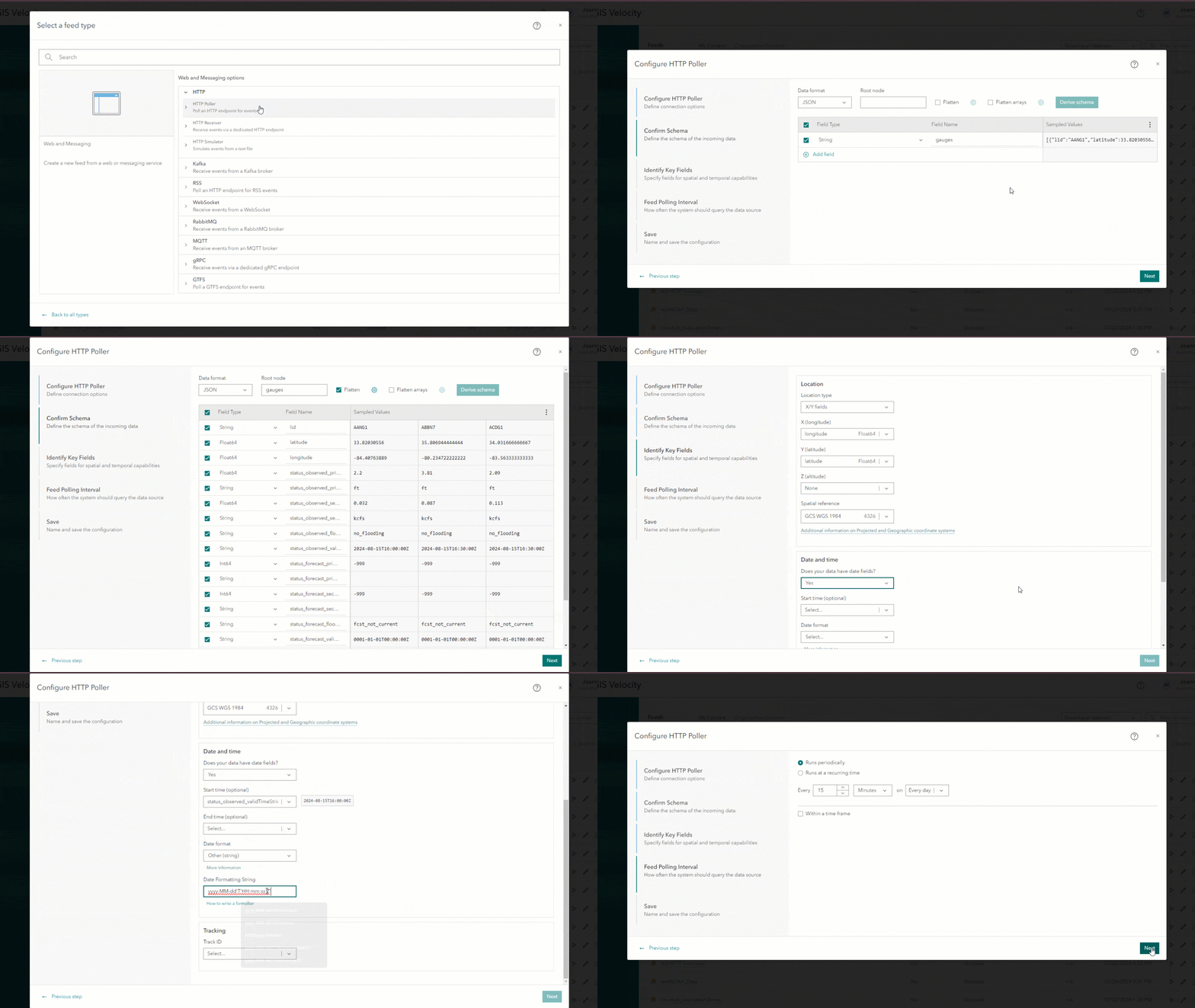
Let’s create a feed that periodically pulls data from the National Water Prediction Service API and brings it into ArcGIS Velocity.

With the ArcGIS Velocity interface open, click “Feeds” and then “+ Create feed.”  Next, expand the option to “See all” under “Web and Messaging,” and then expand the “HTTP” menu and select “HTTP Poller.”  After that, copy and paste the following URL into the URL input for the HTTP Poller:

https://api.water.noaa.gov/nwps/v1/gauges?bbox.xmin=-85.166016&bbox.ymin=33.651208&bbox.xmax=-75.421143&bbox.ymax=36.941111&srid=EPSG_4326

The above URL will query stream gauges from the National Water Prediction Service API. Stream gauges within the bounding box (identified by the bbox parameters) are returned by the query. After that, click “Next.”

The data is returned in nested JSON format. To access the data variables within the nested component, such as the stream gauge latitude and longitude, water heights, etc., specify a root node of “gauges,” and select the option to “flatten” the data. Then, proceed by selecting the “Derive schema” button. These changes will ensure that Velocity only parses data from the “gauges” object, and any other objects within the gauges object are shifted to a single level schema while maintaining the original object(s) names.

After deriving the new schema, we get access to the data variables contained within the nested JSON, which includes a unique ID for each stream gauge in a field called “lid” and each gauge’s current reading in a variable called “status_observed_primary.”  Keep the default field names and click “Next.”

In the Identify Key Fields pane, select “Location type” as “X/Y fields” and choose “longitude” for “X”, “latitude” for “Y,” and GCS WGS 1984 for “Spatial reference.” Then, choose “Yes” for the question “Does your data have date fields” and select “status_observed_validTime” for the “Start time” field.  Next, copy and paste the following date and time format for the “Date Formatting String.”

yyyy-MM-dd'T'HH:mm:ss'Z'

Set the “Track ID” to “lid” and then select “Next.”

For the Feed Polling Interval, set the feed to “Runs periodically” every 15 minutes on “Every day”, then click “Next”. Give the feed a name, such as “streamGaugesNC” and click “Complete.”

Note- This HTTP Poller will return stream gauges that fall within a bounding box which covers North Carolina. Modifying the bounding box parameters will allow you to receive stream gauges for different areas of the United States. You can find more information about querying the API here.

Note- The HTTP Poller feed polls the API every 15 minutes, but this time interval can be adjusted. The minimum poll interval for the HTTP Poller feed is every 10 seconds. While I was investigating the stream gauge data, it appeared that most of the gauges were updating once every 15 minutes, so I opted for the 15-minute poll interval.

Create a Real-Time Analytic

Once you have created your feed, add it to a new real-time analytic. The tools in the real-time analytic will process every feature received from the stream gauge feed.

Step 1: Add and Configure the Filter by Expression Tool

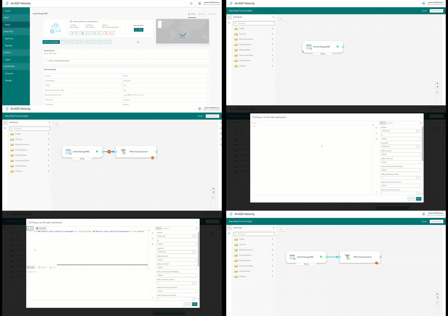
To add and configure the Filter by Expression tool, click the “+” button on the left pane of the real-time analytic, expand the “Manage Data” folder, and then select the “Filter by Expression” tool. Next, drag the output port from the stream gauge feed and connect it to the target port of the Filter by Expression tool.

Double-click the Filter by Expression tool (or right-click  and select “view properties”) to open the tool properties pane. Then, click “Configure an Arcade expression” to open the Arcade code editor. Copy and paste the following Arcade expression into the editor, click “Run” to evaluate the expression, and then select “OK” to complete the process.

$feature.status_observed_primary >= 0 && 
$feature.status_observed_floodCategory != 'out_of_service' && 
$feature.status_observed_floodCategory != 'not_defined'

This Arcade expression in the Filter by Expression tool evaluates the stream gauge data received. We use this tool to remove stream gauges that are returning potentially erroneous data (water height values < 0) or have status values of “out_of_service” or “not_defined.” Select “Apply” to add the Arcade Expression.

Step 2: Add and Configure the Calculate Field Tool

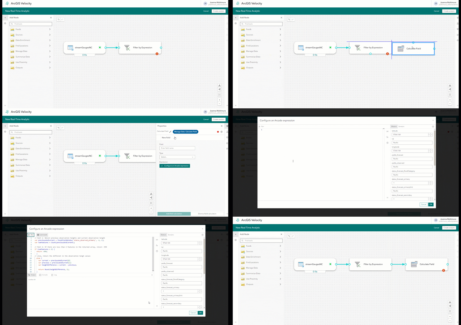
To add and configure the calculate field tool, click the “+” button on the left pane of the real-time analytic, expand the “Manage Data” folder, and select “Calculate Field” tool. Drag the output port from the Filter by Expression tool and connect it to the target port of the Calculate Field tool.

Double-click the Calculate Field tool ( or right-click  and select “view properties”) to open the tool properties pane. Click “Add field calculation” and then click “New field.”  Give the field the name “prevChange” and select “Float 64” as “Type.” Click “Configure an Arcade expression” and copy and paste the following Arcade expression into the code editor.

// Part 1: Return previous observation heights and current observation height
var previousAndCurrent = TrackFieldWindow('status_observed_primary', -1, 1); 
var numFeatures = Count(previousAndCurrent); 

// Part 2: If there are less than 2 features in the returned array, return -999
if (numFeatures < 2) { 
  return -999; 
  } 
// else, return the difference in observation height values
  else { 
    var current = previousAndCurrent[1]
    var previous = previousAndCurrent[0]
    var heightDifference = current - previous;
    return Round(heightDifference, 2);
  }

The above Arcade expression uses a Track Function to access the current water height and previous water height recorded by stream gauges. In real-time analytics, Track Functions enable access to prior observations for the same Track ID.  Track Functions are only supported in the Arcade expression editor of the Calculate Fields and Map Fields tools of Velocity currently. In our case, we will only use the Track Function called TrackFieldWindow, although there are 15 other Track Functions available in ArcGIS Velocity. More information about Track Functions in  Velocity can be found here.

In Part 1 of the above code snippet, we create a new variable called previousAndCurrent, which will store the outputs of the TrackFieldWindow function. The TrackFieldWindow function requires three parameters:

1. A field name (as a string value) that represents the field of interest
2. A start index number, where an index of –1 represents the prior feature (inclusive of this feature)
3. An end index number, where an index of 0 represents the current feature (exclusive of this feature)

In our use of the TrackFieldWindow function, we return the previous observation, which is at a start index of –1, and the current observation, which is at an index value of 0.  Observation values will come from a field called “status_observed_primary” and the outputs from the TrackFieldWindow function are returned in an array called previousAndCurrent.

We then return the count of items in the previousAndCurrent array. Despite stating that we would only return two values from the TrackFieldWindow function (the previous and current observation) why could there be less than two values in our returned array? This can occur if the analytic has not run long enough or if new observations have not been received from the stream gauge.

In Part 2 of the code snippet, we return different outputs based on the count of features in the previousAndCurrent array. We account for situations where the previousAndCurrent array may have fewer than two values by using an if-else statement. If the numFeatures variable is less than two, then we will return a value of –999. However, if the number of items in the numFeatures variable is equal to two, then we create three more variables:

1. var current holds the second item from the previousAndCurrent array (the item at index value 1)
2. var previous holds the first item from the previousAndCurrent array (the item at index value 0)
3. var heightDifference holds the difference between the current and previous stream gauge readings.

Finally, we round the output to return the heightDifference variable with only two digits. This variable is the difference between the current and previous stream gauge height observations.

In the Arcade editor, click “Run” to evaluate the expression, and then select “OK” to complete the process. Select “Add Field Calculation” and then “Apply” to add the Arcade Expression.

Step 3: Add and Configure the Calculate Field tool (again!)

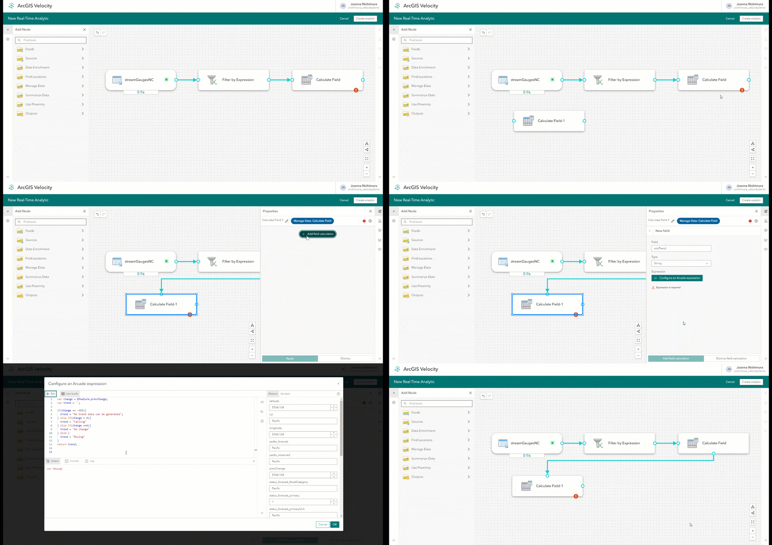
To add and configure the Calculate Field tool, click the “+” button on the left pane of the real-time analytic, expand the “Manage Data” folder, then select “Calculate Field” tool. Next, drag the output port from the first Calculate Field tool to the target port of the new Calculate Field tool. This will add a second Calculate Field tool, which will allow us to access the new field created from the first Calculate Field tool.

Double-click the Calculate Field tool (or right-click  and select “view properties”) to open the tool properties pane. Select “Add field calculation” and then choose “New field.”  Name the field “obsTrend” and select the type as “String.”  Then, select “Configure an Arcade expression,” and copy and paste the following Arcade expression into the code editor:

var change = $feature.prevChange;
var trend = "";

if(change == -999){
  trend = "No trend data can be generated";
} else if(change < 0){
  trend = "Falling"
} else if(change == 0){
  trend = "No change"
} else {
  trend = "Rising"
}
return trend;

The Arcade expression above accesses the output from the previous Calculate Field tool, which is a new field called prevChange. There are four potential scenarios:

1. If the prevChange field has a value of –999, it means there is no previous stream gauge data currently available.
2. If the prevChange field has a negative value, it means that the current stream gauge reading is less than the previous value (the water level is decreasing).
3. If the prevChange field has a value of 0, it means that the current stream gauge reading is the same as the previous value (the water level has not changed between readings).
4. If the above statements are false, then prevChange field must have a value greater than 0, which means that the current stream gauge reading is higher than the previous value (the water level is increasing).

We account for those scenarios in the if-else expression and output results in the trend variable.

In the Arcade editor, click “Run” to evaluate the expression and then select “OK” to complete the process. Select “Add field calculation” and “Apply” to add the Arcade Expression.

Note- Both the calculation for the field prevChange and the calculation for the field trend could be combined into one Calculate Field tool. We decided to split the calculations out into two tools for improved clarity.

Step 4: Add a New Output and Save the Analytic

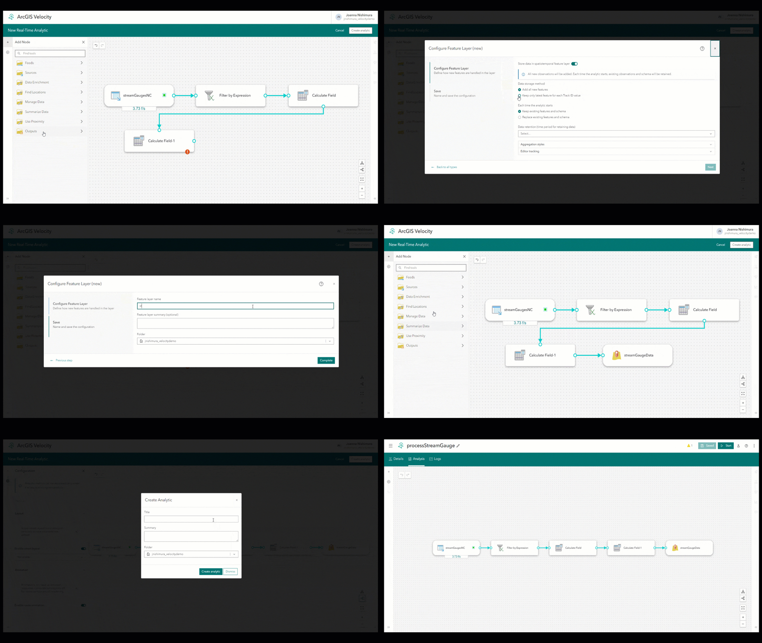
To add a new output and save the analytic, click the “+” button on the left pane of the real-time analytic, expand the “Output Data” folder, then select “Feature Layer (new)” option. Keep the default option to “store data in the spatiotemporal feature layer” and select “Keep only latest feature for each Track ID value” as the Data Storage Method. Choose “Replace existing features and schema” each time the analytic starts. Give the output feature layer a new name, such as “streamGaugeData.”

In the upper right, click  “Create analytic” and enter a new name for the real-time analytic. Next, click “Start” to begin the initialization process, which may take several minutes.

Step 5: Wait for Data…

The HTTP Poller feed is set to return stream gauge data every 15 minutes. Polling occurs at regular time intervals, so if our HTTP Poller is started at 12:08 p.m., the first request for data will occur at 12:15 p.m., the next at 12:30 p.m., and so on. This means that even if the real-time analytic has initialized and is running, there might not be any data returned at that moment from the HTTP Poller feed. So, take a break and check on the analytic later.

After about 45 minutes, I checked the real-time analytic and added the output feature layer to a new web map. Once added to my web map, I disabled the time animations on the layer and enabled the layer to automatically refresh every 0.5 minutes. I set the layer symbology to the field called “obsTrend” and used a blue upward facing arrow for field values of “Rising”, a downward green arrow for values of “Falling”, a horizontal line for gauges with no change, and a square for gauges where “no trend data can be generated.”

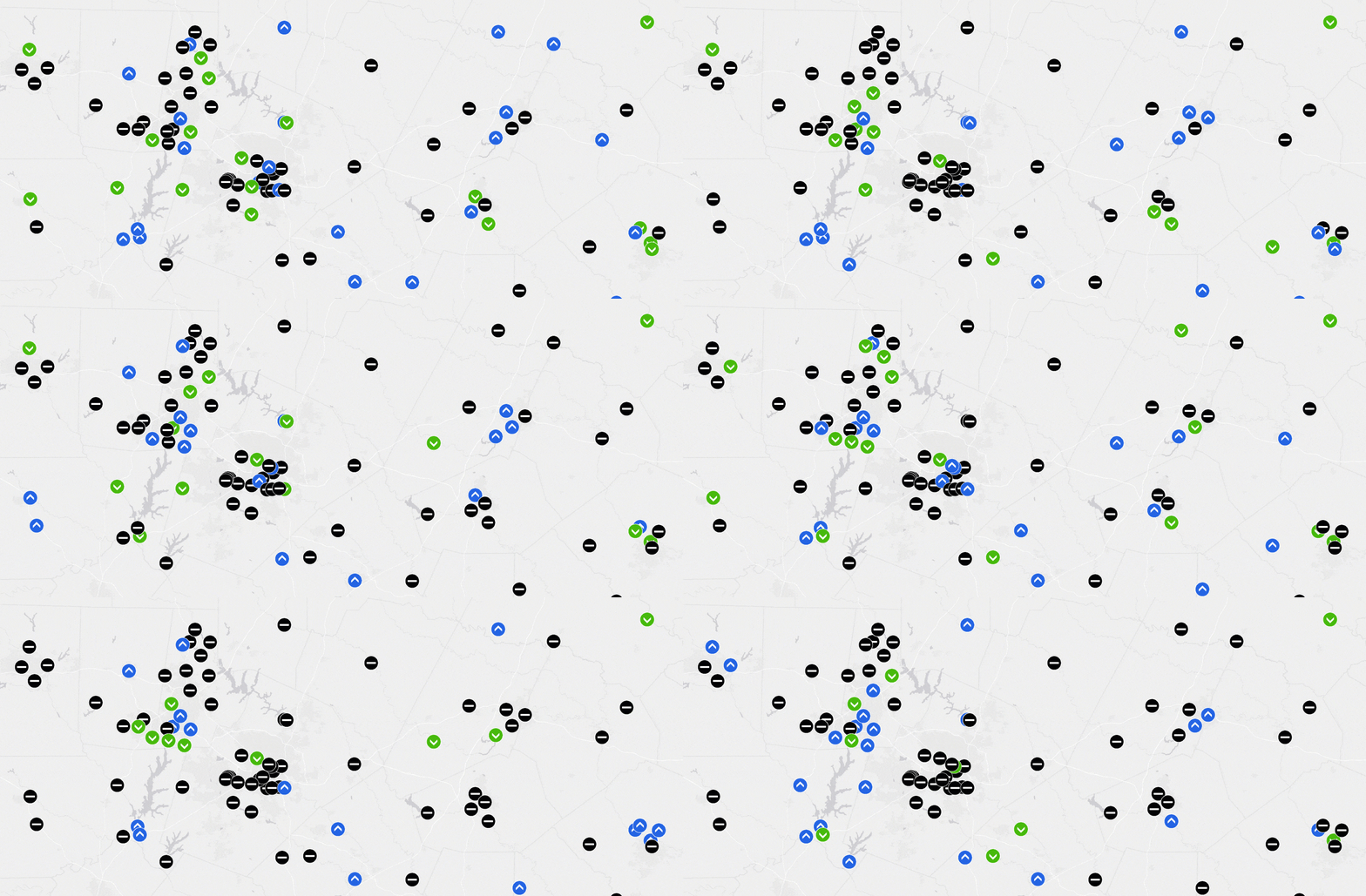
In the event of an emergency, this visualization can help us better understand flood situations by visually tracking the rise and fall of flood waters.

Conclusion

This is just one example of using Track Functions in Velocity. Track Functions provide unique access to historical observations of data, grouped by Track ID and ordered by timestamp. This example used the TrackFieldWindow function; however, there are 15 other Track Functions available in Velocity. Check out this blog to learn about using the TrackGeometryWindow function to access prior geometry values.

To further expand on this current example, I might:

• Add a new TrackFieldWindow field calculation and adjust the time window to return the last four observations. Then, average those observations to get a better understanding of stream gauge height over the last hour.
• Add a new field calculation to calculate the percent change in stream gauge height from the last observation to the current one. Use this calculated value as a second field to symbolize on, allowing us to visualize which stream gauges are increasing or decreasing in height and the magnitude of change.
• Use the Control Event Volume tool with Email output to receive an email notification whenever a stream gauge experiences a notable change in water level between the last observation and the current one.

We are always looking to hear back from the community, if you have any additional questions, please reach out to our team on the ArcGIS Velocity Community.