This article comes with a code sample and demo. Be sure to check it out!
As part of an ongoing effort to support a greater variety of cartographic styling, we recently announced the addition of gradient symbology to the ArcGIS Maps SDK for JavaScript. Gradient fills and strokes are powerful options for CIM symbols that make it possible to create all kinds of expressive symbology:

This article takes a look under the hood at the implementation of gradient strokes. It will outline the overall strategy as well as highlight some details of the underlying WebGL logic.
Gradient strokes are a way to style lines in Esri’s Cartographic Information Model (CIM). They transition from one color on one side of the line, to another color on the other side of the line. Gradient strokes are a flexible tool that can create a wide range of cartographic effects. Esri’s John Nelson has made some excellent guides showing how you can use gradient strokes to represent the banks of a river, peel up an area of interest, or shine a spotlight on a feature!
Here’s a section of Tōtaranui / Queen Charlotte Sound symbolized with a gradient stroke:
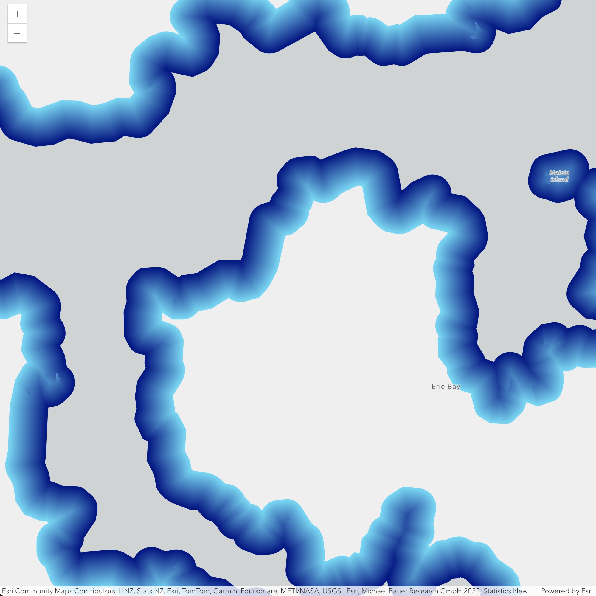
So how does this work in the JavaScript Maps SDK? The core idea is relatively straightforward: for each pixel covered by the line, calculate the distance from the edge of the line, and then use that distance to get a color from the gradient.

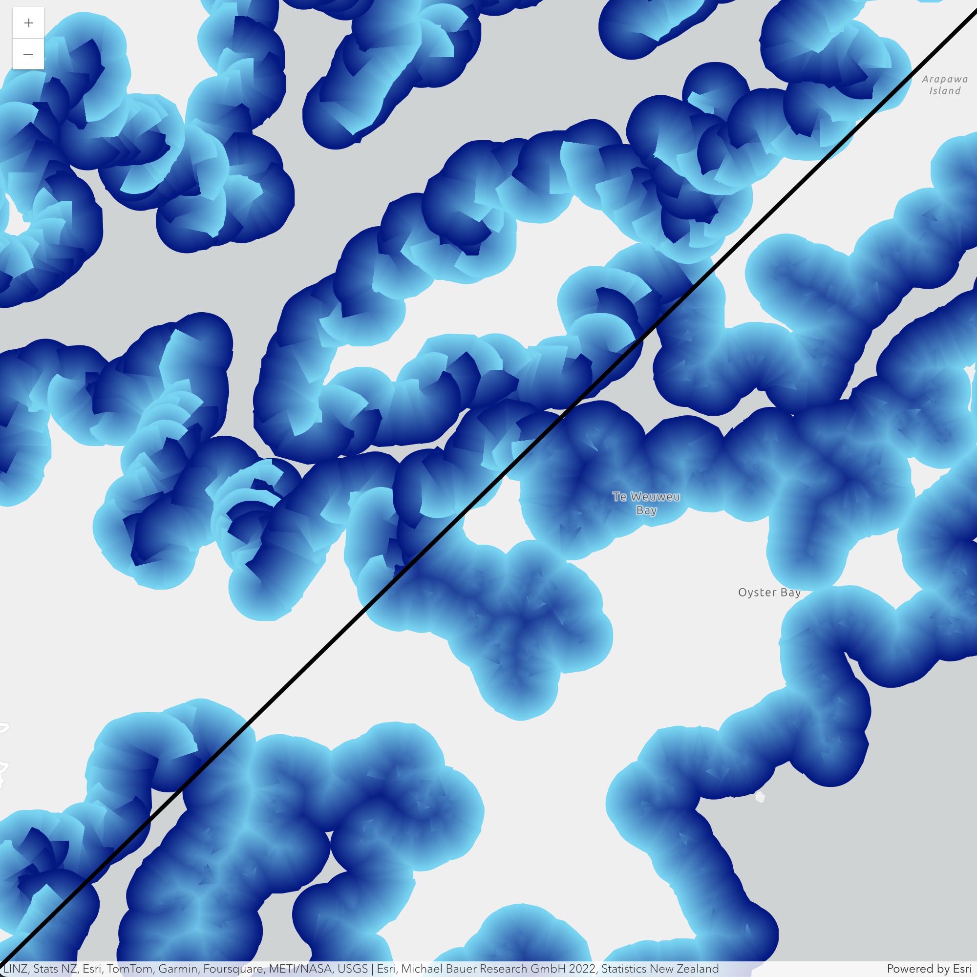
This works well for simple shapes, but what about complex polylines or clusters of features? Drawing each line as its own separate gradient would produce something like this:
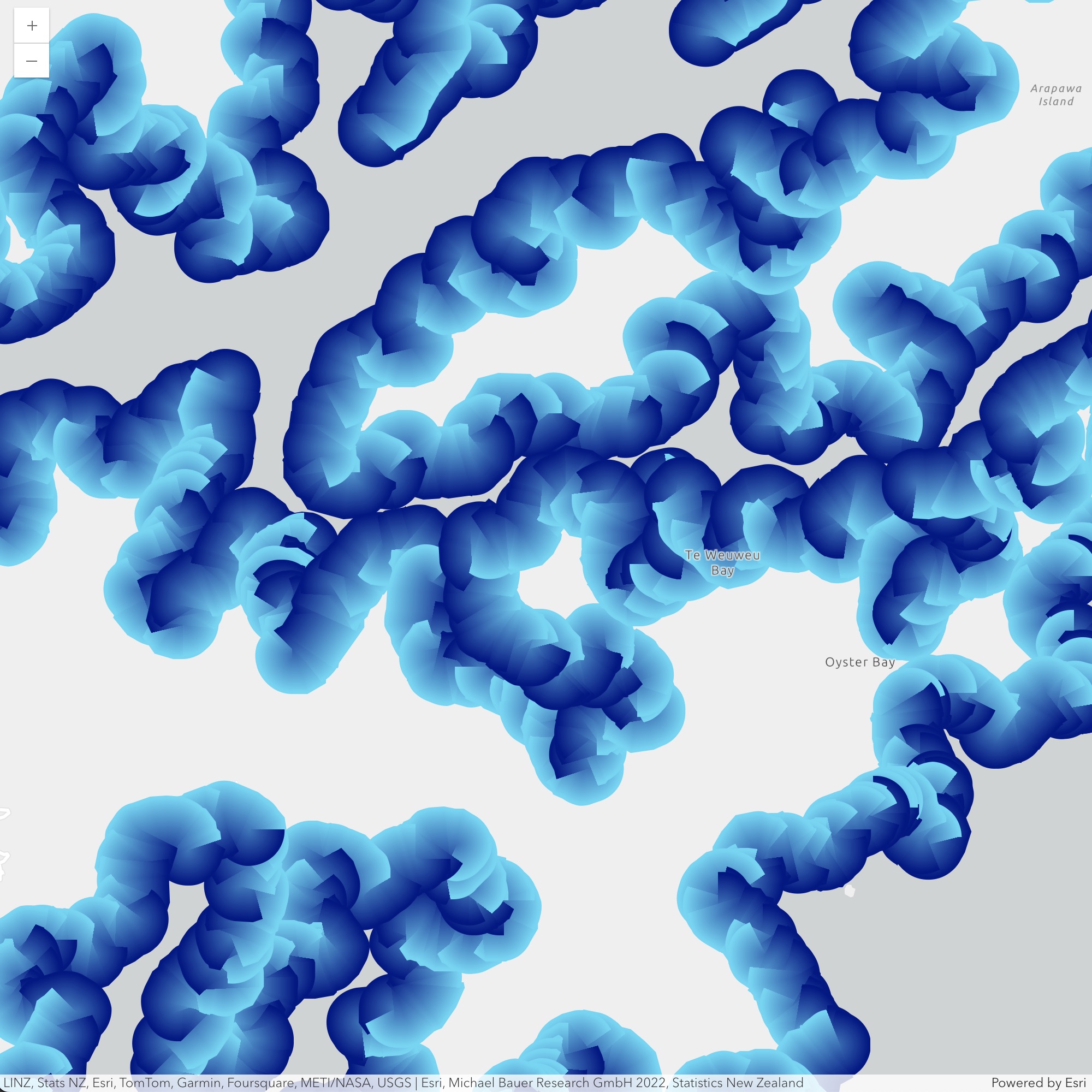
What’s happening here is that each line segment is being drawn as an independent rectangle with a gradient. When two rectangles overlap, one is drawn directly on top of the other, creating a visual discontinuity in the gradient. We’d prefer for these overlapping gradients to resolve into a single smooth buffer. To do so, we’ll have to dive into the rendering code.
The JavaScript Maps SDK uses WebGL to render large amounts of data at interactive speeds in the browser. WebGL is a Javascript API built into all major browsers that allows web apps to run code directly on the computer’s graphics processing unit, or GPU. Because the GPU is able to process lots of data in parallel and can quickly output pixels to the screen, libraries like the JavaScript Maps SDK use it to run calculations and display shapes and images in real time.
While WebGL can draw lines directly, its ability to do so is fairly limited, and in practice lines are most commonly drawn using sets of triangles. Each point on the line can be split into two points, a left and a right (or an inside and an outside), which are extruded away from the centerline. These extruded points are then connected up to form triangles.
For a great writeup on line representation and rendering, see my colleague Dario D’Amico’s blog post about animated flow lines as well as his sample describing custom WebGL animated lines, which is where I got this nifty animation.

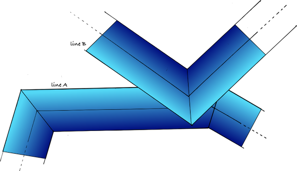
Triangles (made up of extruded points) contain a lot of useful information for rendering the line. By interpolating between the extrusion vectors, we can calculate each pixel’s distance from the edge of the line segment, which determines what color to pick from the gradient. But we can also calculate each pixel’s distance from the centerline of the line segment, which, it turns out, can help fix the problem of overlapping gradients.
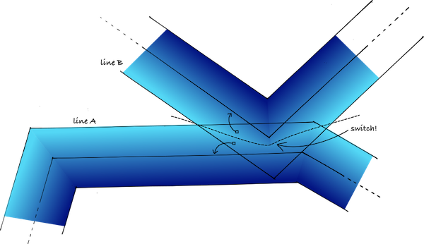
Currently when two lines, “A” and “B”, are near each other, line B simply draws directly on top of line A. What we want is to switch from drawing line B to drawing line A halfway between the two. In other words, we want each pixel to only draw the gradient from the line that it’s closest to.
There’s a trick we can use to accomplish this with WebGL. Like most graphics APIs, WebGL provides support for something called depth testing. For each triangle that covers a given pixel, the GPU generates (at least conceptually) what’s called a fragment, which contains information about that particular pixel for that particular triangle. Depth testing allows you to assign a numerical value, called a “depth”, to each fragment, and then reject certain fragments based on their depth values.

The real advantage of depth testing is that rejecting fragments lets the GPU avoid unnecessary work. Imagine a 3D scene of a table covered by a tablecloth. Without depth testing, the GPU would have to do all the work of drawing the table, which could be quite expensive, even though we won’t be able to see the results of all that work because the table fragments are obscured by the tablecloth fragments. If instead we draw the tablecloth first, we can use depth testing to skip over all the fragments from the table.
In the case of gradient strokes, depth testing can’t provide any performance speedups, but it can help us choose which gradient to draw at each pixel. Remember that we can use the interpolated extrusion vectors to calculate the distance from each fragment to the center of its line. This is the trick: all we have to do is to feed that distance into the depth test, and tell the depth test to keep the fragment with the lowest distance. That way, each pixel will draw only the gradient from the line it’s closest to.
Here’s an image showing before and after this depth testing approach is applied. There are still a few artifacts due to the complexity of the data, but you can see that the many overlapping gradients are largely being resolved into one.
If you’re familiar with signed distance fields, you might recognize this kind of visualization. A distance field is a raster where each pixel contains the distance to its nearest “obstacle” — often a shape or object in frame. A common variant is the signed distance field (SDF), which uses positive and negative values to differentiate pixels that are inside the obstacle from ones that are outside. Distance fields are a very common data structure with a wide range of applications including in image processing, robotics, and computer graphics. The JavaScript Maps SDK uses SDFs to draw things like markers, text, and dashed lines.
It turns out that the method outlined above is a handy one-pass technique for generating signed distance fields on the GPU. The easiest way to achieve this effect from scratch is to triangulate each path segment with two end caps.

This particular layout makes it simple to interpolate the vertex extrusion vectors and signs in order to calculate a per-fragment signed distance that can be used for depth testing and visualization. If you use very wide lines, you can cover the entire frame, producing a complete SDF. Here’s a standalone demo showing how it works. You can also find a slightly simplified version here.

It’s worth mentioning however that this technique is not entirely suited to full-screen SDF generation; there are some technical caveats. First, the depth must be written from the fragment shader in order for interpolation to run correctly, which precludes early depth testing. Second (and as a result), compared to screen-space techniques like jump flooding, this approach saves on draw calls and sampling by sacrificing heavily on overdraw. And finally, it struggles to handle the sign of the distance for contiguous or intersecting shapes.
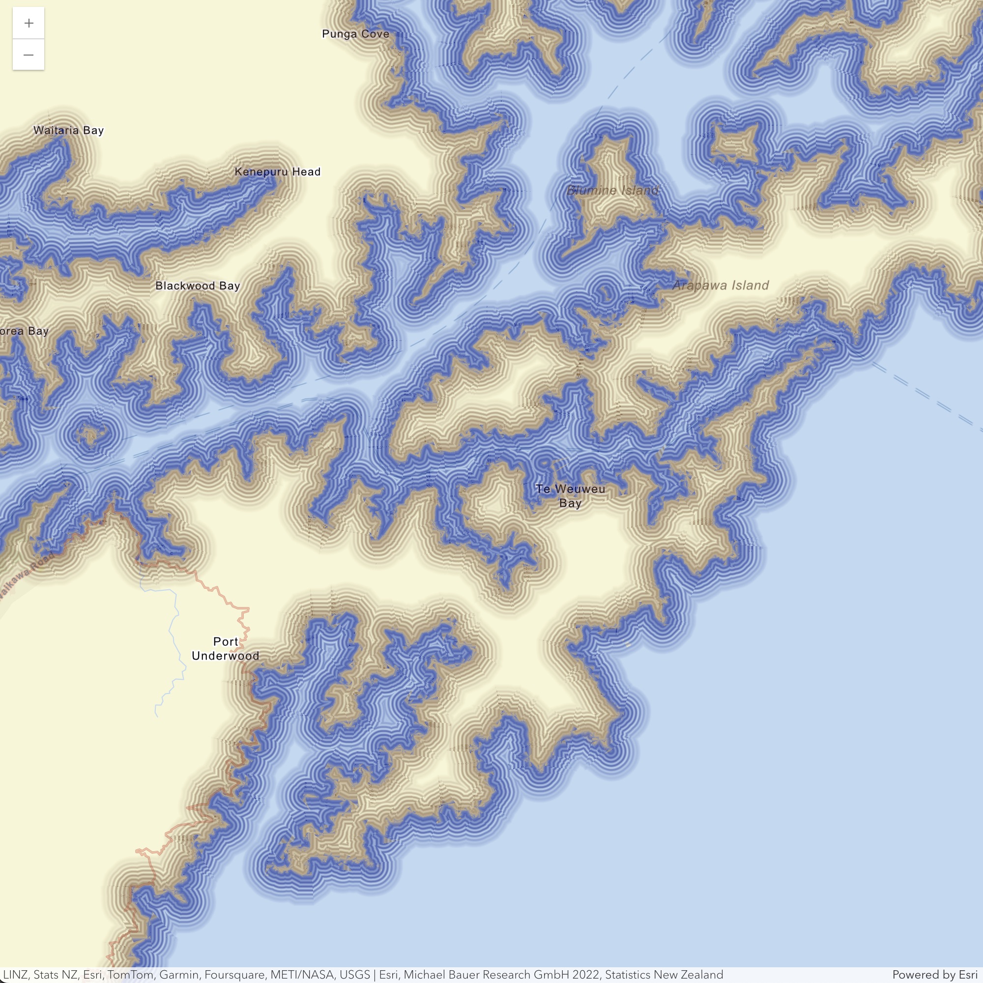
We use a slightly modified version of this approach to render gradient strokes in the JavaScript Maps SDK. And now that we understand how the technique works, we can use it to create all kinds of interesting cartographic effects. Here’s a larger region of Tōtaranui / Queen Charlotte Sound, this time visualized with a multistop gradient stroke showing isolines of equal distance, where color represents the sign of the distance.
Hopefully you enjoyed this deep dive into gradient visualization in the JavaScript Maps SDK. Happy coding and happy mapping!
For additional reading, please visit the following links:
- Draw complex polygons in ArcGIS Pro, super fast by John Nelson
- Visualize and animate flow in MapView with a custom WebGL layer by Dario D’Amico
- Implementation of feature highlights in the ArcGIS Maps SDK for JavaScript by Dario D’Amico
- A trip through the Graphics Pipeline 2011 by Fabian Giesen
- Signed distance functions (Wikipedia)

Article Discussion: