ArcGIS for Power BI join layer improvements

ArcGIS for Power BI 2024.2 introduces several improvements to the join layer feature. These improvements include highlight interaction (in addition to filter), styling of the joined result layer, and appended join layer fields as part of the feature information widget.

If you’ve used join layers before, you may be aware of the added capabilities it brings when your Power BI data lacks location information. These capabilities were described in the No location? No problem! Join layers in ArcGIS for Power BI blog article.

You don’t need experience using join layers to follow along with this blog article, however. You’ll start with a basic join layer example, using sample data and a public feature layer allowing you to create the example yourself and follow along as you read the article. In further examples, you’ll explore existing capabilities and improvements. And finally, you’ll learn additional recommendations and caveats for using the join layer feature.

The following sections will guide you through these topics:

• Create a join layer using the new user interface
• Use the filter and highlight interactions
• Understand join operations: Select first row only and Aggregate
• Appended join layer fields: Feature information, exploring aggregation, and statistic types
• Appended join layer fields: Styling the joined result layer and labels
• Join layer and related feature layer on the map
• Recommendations
• Caveats

Create a join layer using the new user interface

Before creating the join layer, take a look at the sample data. Download and view the following file: mock_customer_data.csv. It includes the following fields: id, first_name, last_name, email, city, state, latitude, longitude, amount, and probability.

Keep the following in mind:

• The data is automatically generated mock data—any similarities to real persons or locations are unintentional.
• Latitude and longitude are references to city locations.
• All U.S. states are represented in the data except Maine and South Dakota.
• Field id represents a unique ID for the dataset.

To begin the example, upload the .csv file in Power BI Service (or Desktop) to create a semantic model, and then create a blank report using the semantic model. For more detailed guidance on this step, refer to the Get data from comma separated value (CSV) files topic in the Microsoft help.

To create a join layer, complete the following steps:

1. Click the ArcGIS for Power BI visual to add it to the report page.
2. Sign in as an ArcGIS user or continue as guest.
   The examples in this article do not require an ArcGIS user account.
3. Drag the state field to the Join layer field well.
4. Click the Go to Join layer link in the message.

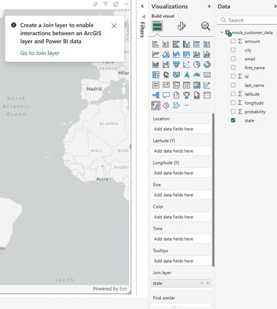
The Join layer tool tab opens on the Analysis pane.

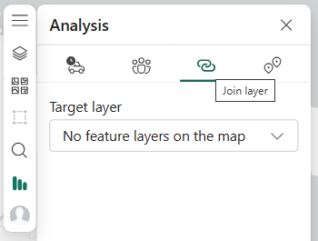
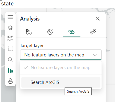
5. On the Target layer drop-down menu, select Search ArcGIS.

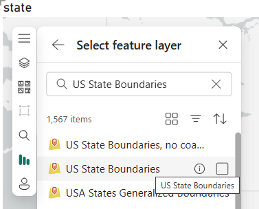
6. Search for US State Boundaries and select the US State Boundaries feature layer from the result by checking the check box.
   If signed in as an ArcGIS user, search in the ArcGIS Online category.

6. Select fields displays and the Power BI data field state is preselected under Power BI data.
7. Select the feature layer matching field NAME under Feature layer.

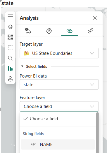
1. At this point, the join layer is ready to be created, but before you click Create join, take a closer look:
   1. 1. After choosing a field, you’ll notice an Estimated match accuracy section. This is an indicator of how well the data matches using sample data. Each time you add a field and select a matching feature layer field, this will be recalculated.
      2. The Result layer section has more options. The default values for each option, shown below, are explained further in the following section.
      3. The default result layer name is the combined title of the feature layer and the Power BI dataset name. Change this name to Join layer. You can also rename it later in the Layers pane.

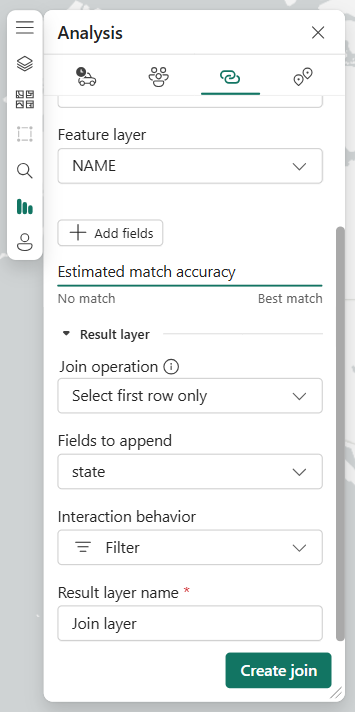
8. Leave the default values in Join operation, Fields to append, and Interaction behavior for now.
9. Click Create join to create the join layer.
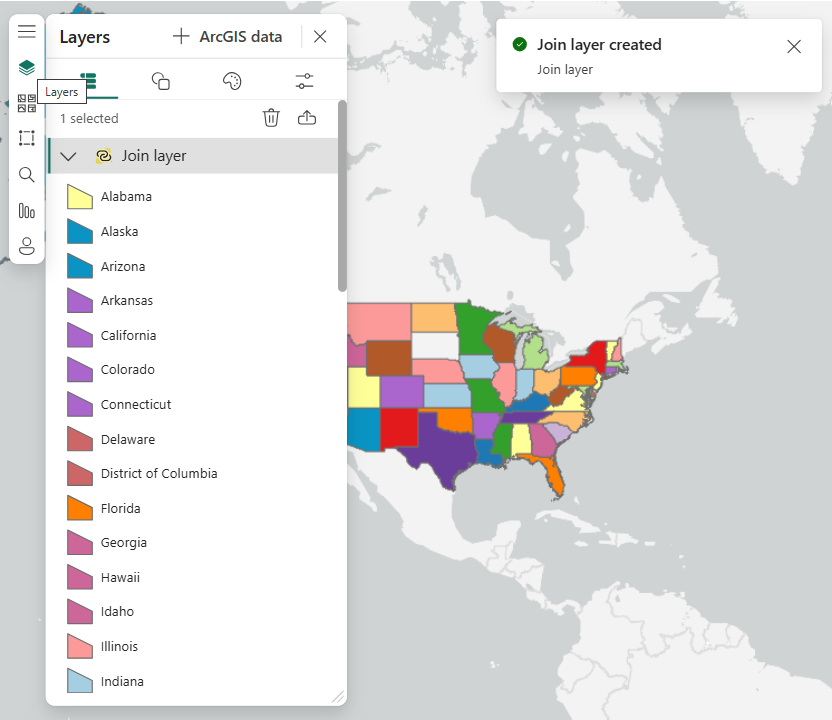
   A Join layer created confirmation message is displayed.
10. Open the Layers pane from the toolbar.

11. Click the Expand button to show the join layer’s legend.
    Note: The join layer’s legend will be based on the original feature layer legend. Later, you’ll explore how to modify the legend by styling the join layer.
    Note: The states Maine and South Dakota are not in the legend, and they are not rendered on the map. These states aren’t represented in the Power BI data as mentioned above.

12. Close the Layers pane and the Join layer created message.

Use the filter and highlight interactions

In the Join layer tool, the default interaction behavior is Filter.

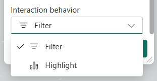
Filter was the only interaction behavior for the join layer in previous releases of ArcGIS for Power BI. In this release, the Highlight interaction is also available.

Use the Filter interaction

To use the Filter behavior, add an external visual to the report:

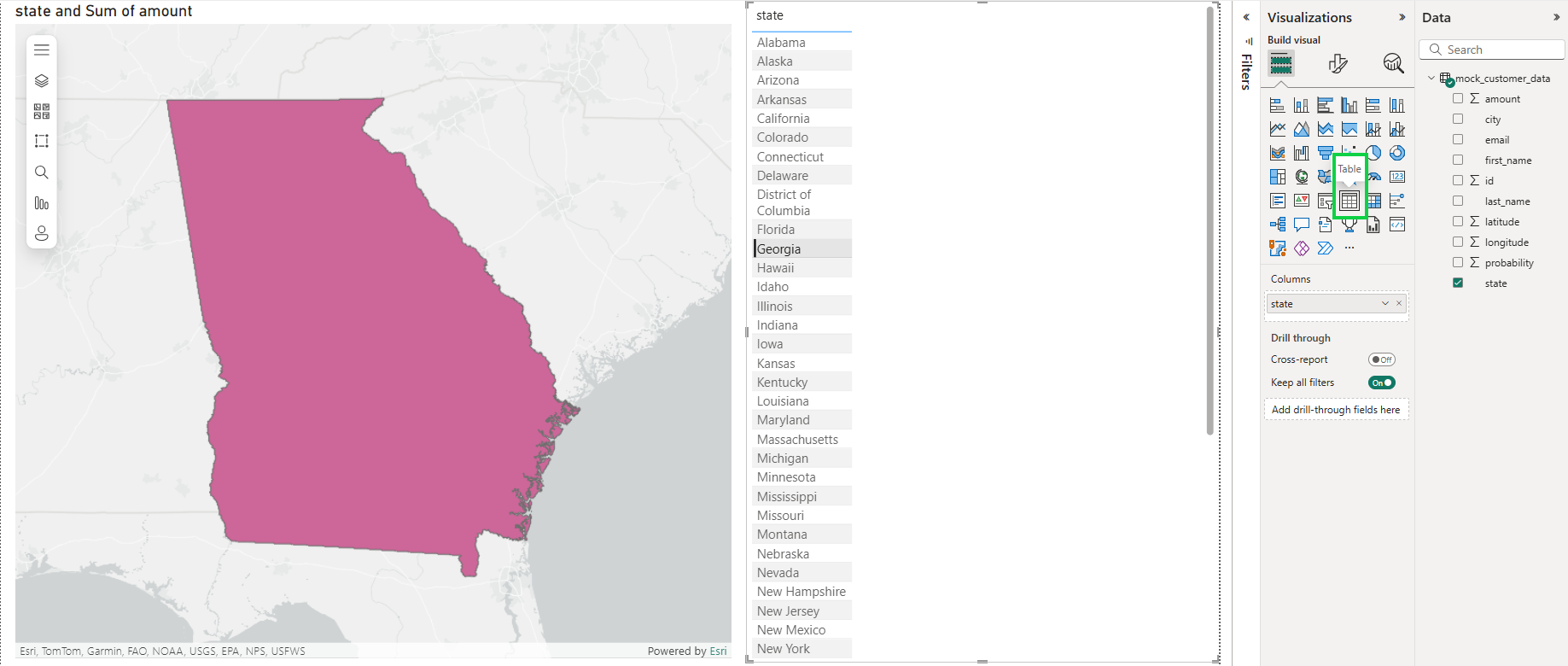
1. Click on a blank area outside the map and then click on the Table visual to add it to the report.
2. Drag the state field to the Table visual Columns field well.
3. Click the state of Georgia in the Table visual on the report page.
4. Notice that the map renders only the selected state and filters out all others.
   The map also zooms in to focus on the selected state.

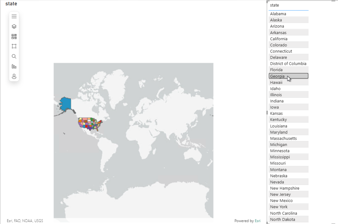
5. Click the state of Georgia again in the Table visual to deselect.
6. Notice the filter is removed, all states are rendered, and the map zooms back out.

1. Tip: When Filter is the interaction behavior, you may not want the map to automatically zoom in and out when selecting and deselecting features. To configure this, do the following:
   1. 1. 1. Select the map.
         2. Zoom (using the mouse scroll wheel) and pan (click then drag the mouse) until the map shows the 48 contiguous U.S. states.
         3. Under Visualizations, click the Format your visual tab.
         4. Under Visual, expand Map controls.
         5. Turn on Lock Extent.
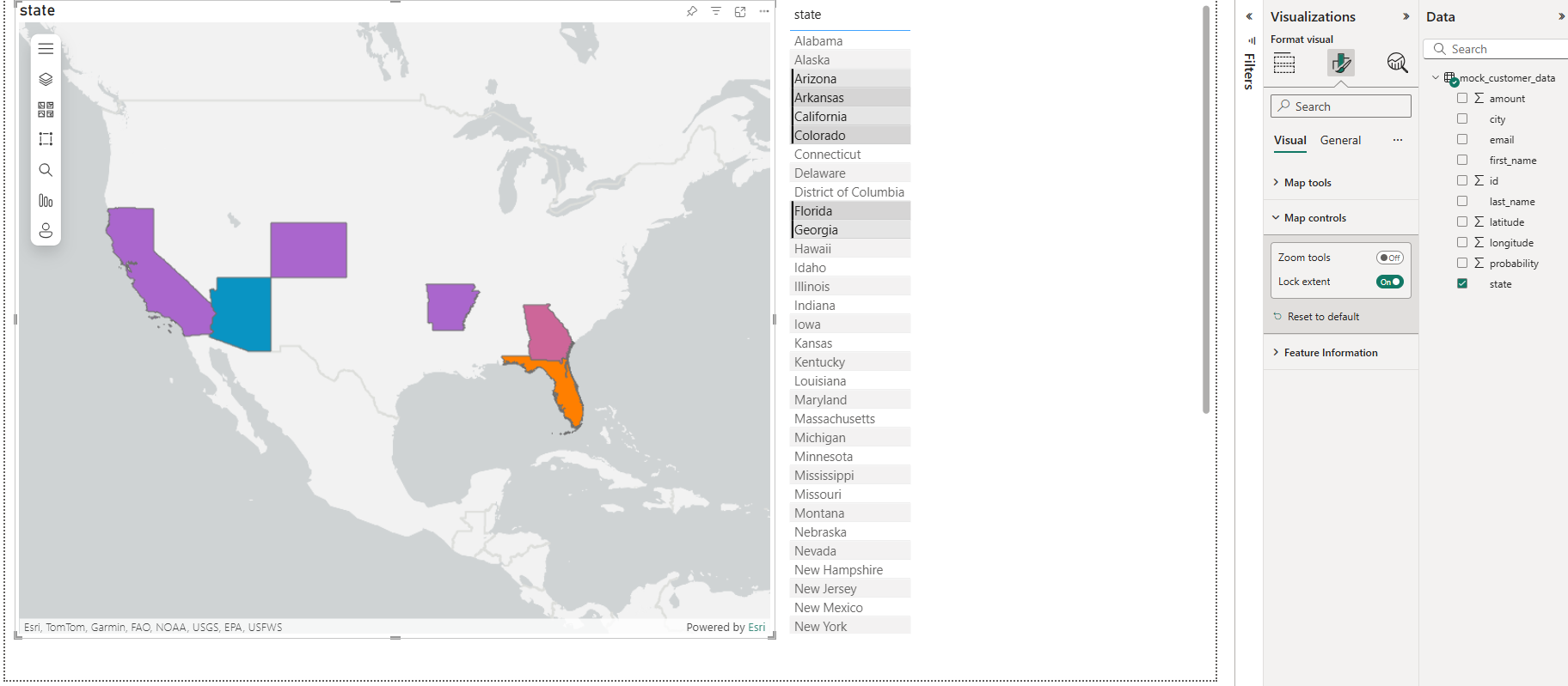
            This prevents the automatic zoom on selection.
         6. Select and deselect multiple states in the Table visual and notice the filter interaction in the map.
            Selected states are filtered, but the map will no longer zoom in and out.

Use the Highlight interaction

To use the Highlight behavior, complete the following steps:

1. Open the Analysis pane from the toolbar.
2. Select the Join layer tab.

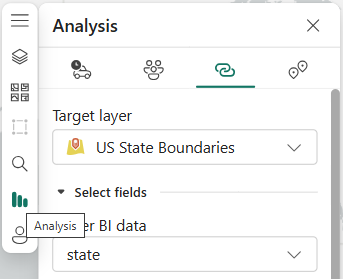
3. Scroll down to Interaction behavior and select Highlight.

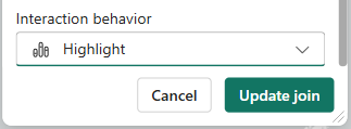
4. Click Update join.
   A message displays to show the join layer was updated.
5. Close the Join layer tool and the Join layer updated message.
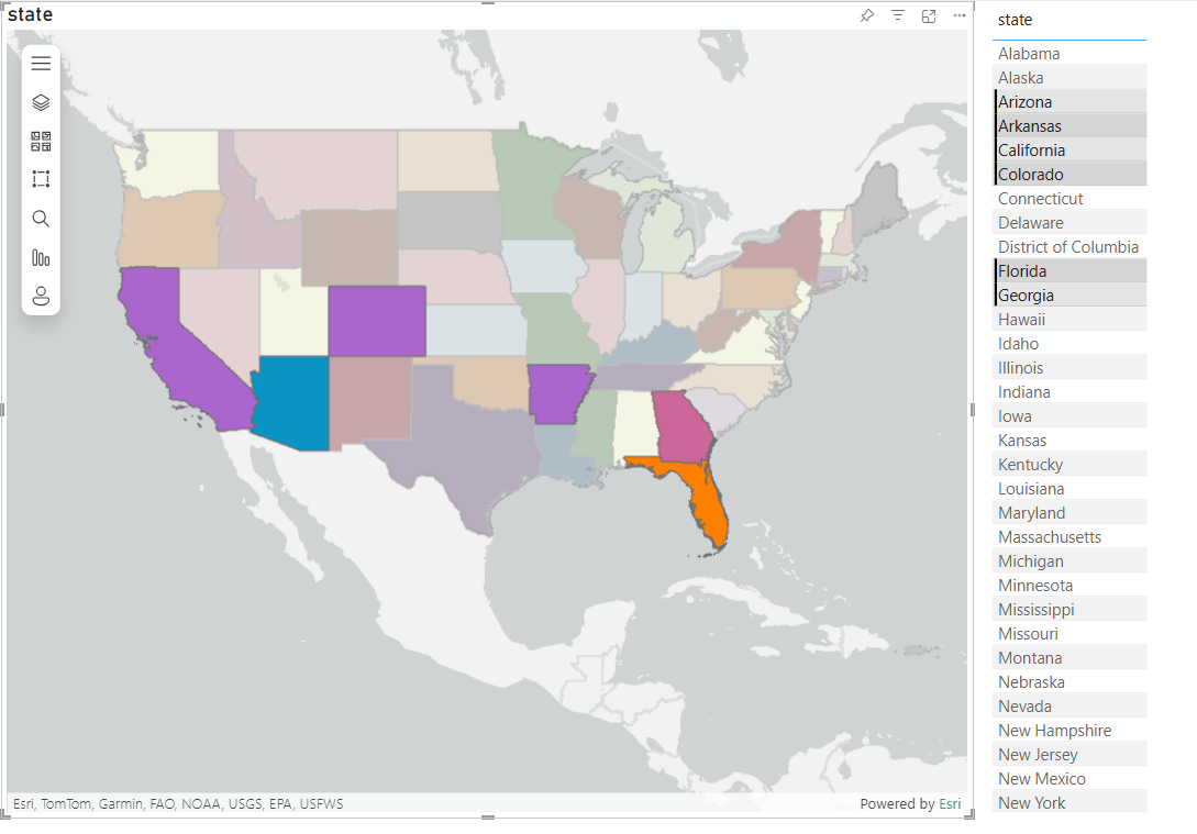
6. Select and deselect multiple states in the Table visual.
7. Notice that the map renders all states but highlights only the states selected in the Table visual.
   Note: Because all joined features are rendered using the highlight interaction, the map won’t automatically zoom in and out to the selected features.

Understand join operations: Select first row only and Aggregate

When joining feature layer data to the Power BI data, you have two options: Select first row only or Aggregate. To choose, you must understand the nature and aggregation aspects of the Power BI data and how they relate to the feature layer data to which it is being joined.

Aggregation of Power BI data

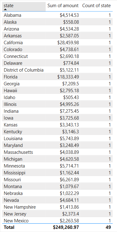
In Power BI, you can view data aggregation quickly using the Table visual. Before returning to the Join layer tool in the ArcGIS for Power BI visual, view some aggregation result examples in the Power BI Table visual by selecting combinations of data in its columns. You can adjust the Table visual on your report using the same fields from the sample data.

Aggregation example 1 uses fields state, Sum of amount, and Count of state (distinct).

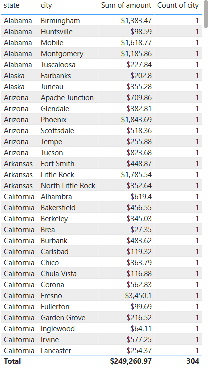
Aggregation example 2 uses fields state, city, Sum of amount, and Count of city (distinct).

Aggregation example 3 uses fields state, city, id, Sum of amount, and Count of id (distinct).

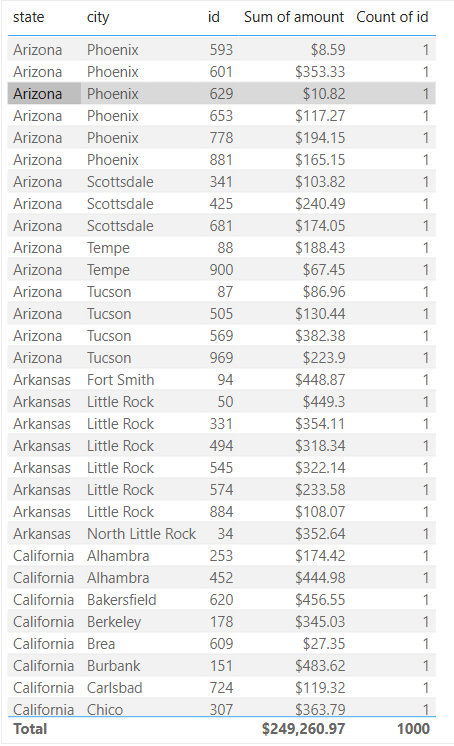
Each example summarizes or aggregates data at a different level, and each contains a different number of records. This all depends on the fields added to the visual’s field wells. The same aggregation of data is true for the ArcGIS for Power BI visual. As you add fields to the field wells, Power BI supplies the visual with this updated data, which can then affect how that data is joined to the join layer’s feature layer. This impacts the cardinality of the join.

Example 1 is aggregated at the state level and has only 49 records.

Example 2 is aggregated at the city level and has 304 records.

Example 3 is aggregated at the ID level (which is the unique key of data) and so it contains all 1,000 records of the dataset.

When using an ArcGIS feature layer that represents U.S. states (state being the key value), you would expect the join to data from example 1 to be 1:1.

Joining that same ArcGIS feature layer to data from examples 2 and 3, you can expect the cardinality to be 1:n.

Note: When referencing cardinality in the ArcGIS for Power BI visual, the ArcGIS feature layer is on the left and the Power BI data is on the right.

Learn how aggregation works in a join layer

Return to the example, with only the state field added so far.

1. Open the Join layer tool.
2. Scroll down to the Result layer section of the tool.
3. Ensure you don’t have any current selections or filters applied using the Table visual or the Filters pane.
4. Click the Join operation information button .
   Note: Feature layer to Power BI cardinality is 1:1.

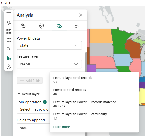
5. Click the Join operation information button again to remove the pop-up.
6. Now drag the city field to the Join layer field well.
7. Click the Join operation information button again.
8. Notice the Join layer updated message indicating an aggregation change, the Power BI total records changed, and the cardinality is now 1:n.

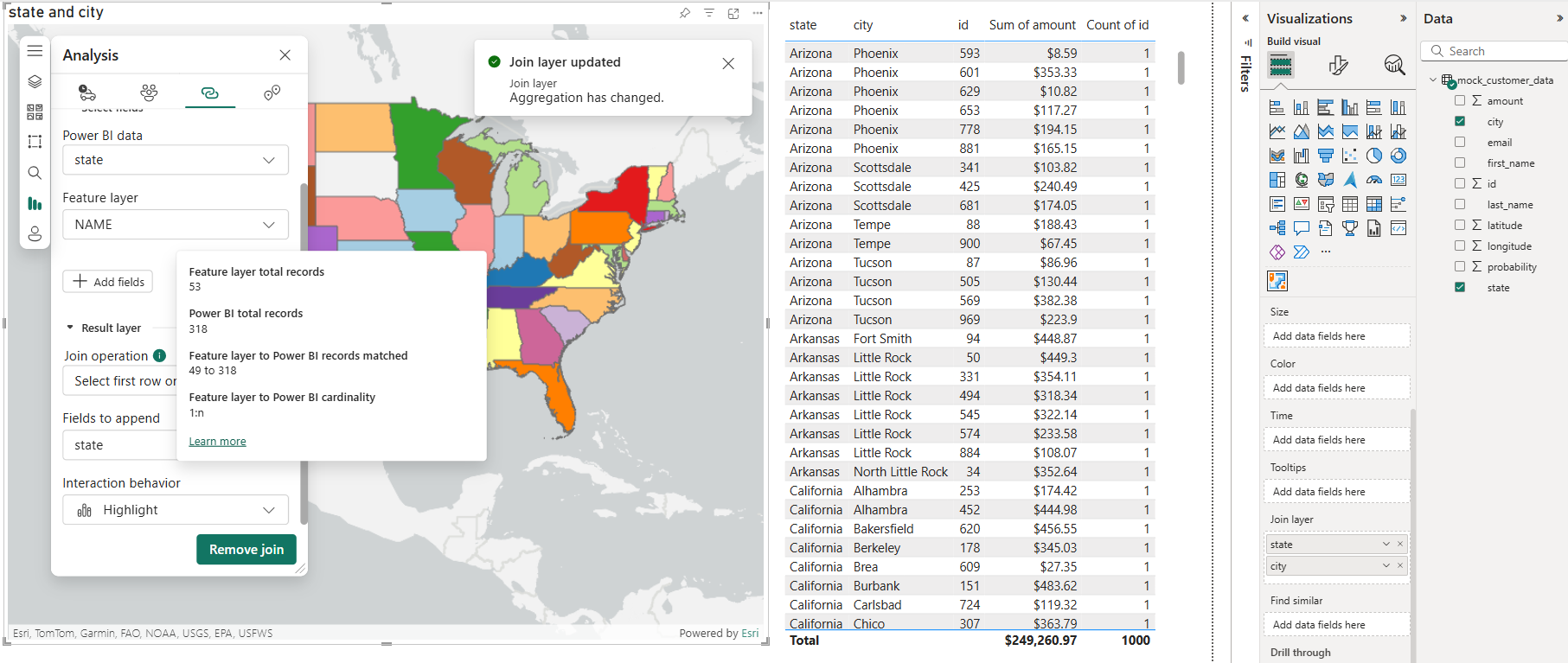
These examples are to illustrate that adding fields to any field well can change the cardinality of any existing join layer you have already created.

Explore the join operations options in ArcGIS for Power BI

On the Join operations menu, Select first row only is the default value and makes the most sense if the join cardinality is 1:1 and you know that the row data joined on both sides of the join represents unique values. If the join cardinality is 1:n, the recommended choice is Aggregate. The Join operation choice will also change which fields are available on the Fields to append drop-down menu.

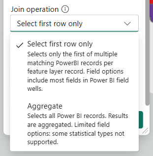
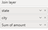
1. Add field Sum of amount in addition to fields state and city to the Join layer field well.

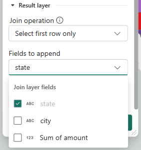
2. Choose Select first row only for the Join operation in the Join layer tool.
3. Click the Fields to append drop-down menu and notice the field choices.
   The state field has already been selected.
   All key fields in the join definition (under Select fields) will automatically be included in the Fields to append list.
   All other fields added to field wells will also be available for selection.

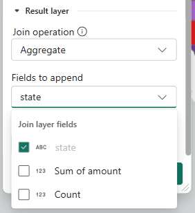
4. For Join operation, choose Aggregate.
5. Click the Fields to append drop-down again and notice the change in field choices.
   The field city is no longer an option, because when you choose Aggregate only numeric or statistical fields can be appended.
6. Notice another field, Count.
   This is a calculated field that is always available when choosing Aggregate.
   This represents the total count of Power BI data records found matching each feature record in the ArcGIS feature layer.
   You’ll use this field in the next section.

Appended join layer fields: Feature information widget, exploring aggregation, and statistic types

When you append additional join layer fields, there are several useful applications for these fields. You can view the appended data in the feature information widget. You can use the appended fields to style the layer. And you can use the fields in labels.

Use the Feature information widget

To see the results in the feature information widget, start by updating the join layer.

1. Ensure you have state, city, and Sum of amount fields in the Join layer field well.

2. Open the Join layer tool.
3. For Join operation, select Aggregate.
4. Click the Fields to append drop-down menu and select Sum of amount and Count.

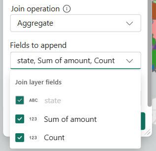
5. Click Update join to update the join layer with the new fields.
6. Close the Join layer tool and the Join layer updated message.
7. Update the Table visual.
   • For reference, ensure the Table visual on the right is using the state, Sum of amount, and Count of city (distinct) fields.
8. Select the ArcGIS for Power BI visual and open the Format visual tab.
9. Expand Feature Information under the Visual tab.
10. Click Enable.

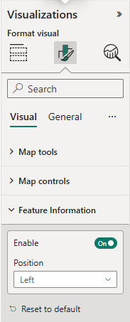
11. On the map, expand the Feature Information pane.
    The Feature information pane appears on the left side of the map by default.
12. Expand the Feature information pane.
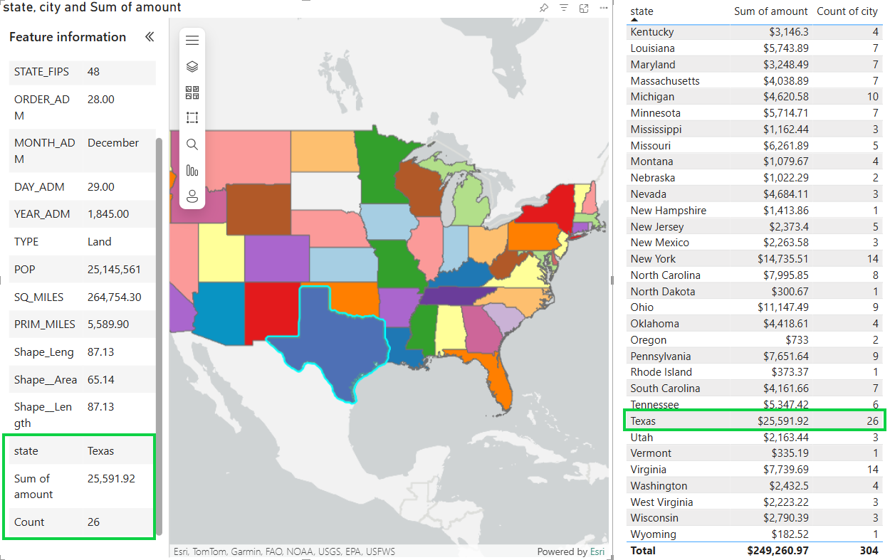
13. Click the state of Texas on the map.
14. Scroll down in the Feature information pane.
    The last three fields are the fields in the join layer’s Fields to append section.
    The Count field represents the count of distinct cities found in the supplied Power BI data that matches the feature (Texas).
    This is because the categories included in the data are state and city.
    The Count field values in any given join layer using the Aggregate join operation will represent the level of aggregation created by the fields added in all field wells (not just the Join layer field well).

Explore aggregation

You can change the aggregation by adding the id field.

1. Add the id field to the Join Layer field well.
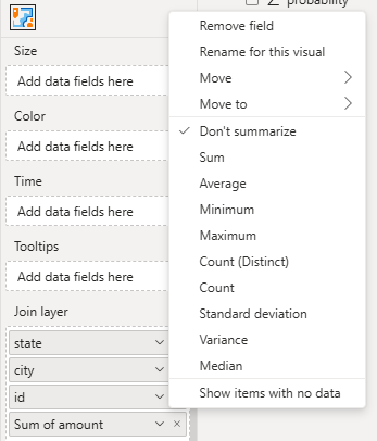
   • Note: By default, id will change to Sum of id because it is numeric. Switch to Don’t summarize by clicking the down arrow next to field Sum of id.
   • TIP: Whenever you add a numeric field to the Join layer field well, it will default to Sum and operate as a statistical value. If your intent is to use that field as a key field in the join definition, you should always switch to Don’t summarize. If your intent is to use it in Fields to append as a statistical value, you can leave it as Sum or one of the other statistical options.

1. You will see a Join layer updated message indicating an aggregation change.
2. Close this message.

3. Update the Table visual.
   • For reference, ensure the Table visual is using fields: state, Sum of amount, and Count of id (distinct).
4. On the map, click the state of Texas again.
5. Scroll to the bottom of the Feature information pane.
6. Note the value of the Count field is now 100.
   This is because the categories to aggregate now include state, city and id, with id being the lowest level of aggregation.
   The Count value now represents the distinct number of ids in Texas.

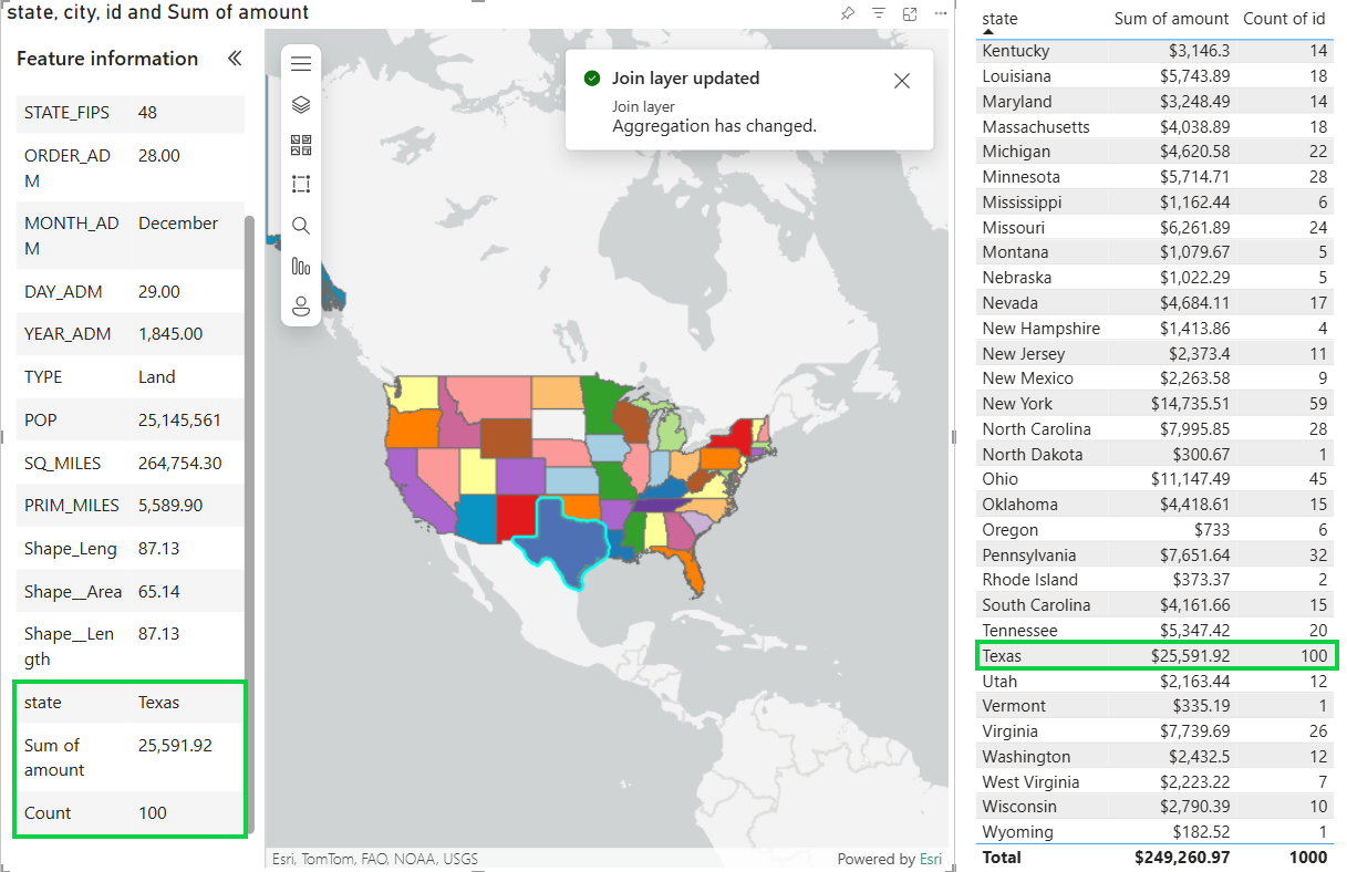
The above examples illustrate why it is important to take notice when aggregation has changed due to adding fields to field wells, and how that aggregation can impact your join layer results.

Explore statistical types

When you use Aggregate as your join operation, only some of the Power BI statistical types are supported when used in Fields to append for a join layer: Sum, Minimum, Maximum, and Count. If you change the statistical type of a field after the join layer has been created, the join layer will be updated. If you change it to an unsupported statistical type, the join layer updates, and that field will be removed from the join layer.

1. Remove the id field that you previously added.
   A Join layer updated message appears.

The Join layer field well now looks like this:

2. Open the Join layer tool.
3. Ensure Join operation is set to Aggregate and the Fields to append options are state, Sum of amount, and Count.
4. Update the join if necessary.

5. Leaving the Join tool open, change the statistic type on the Join layer field well from Sum of amount to Maximum.
6. Notice the join layer is updated due to a statistical type change.
   The field name is changed and is reflected in Fields to append.

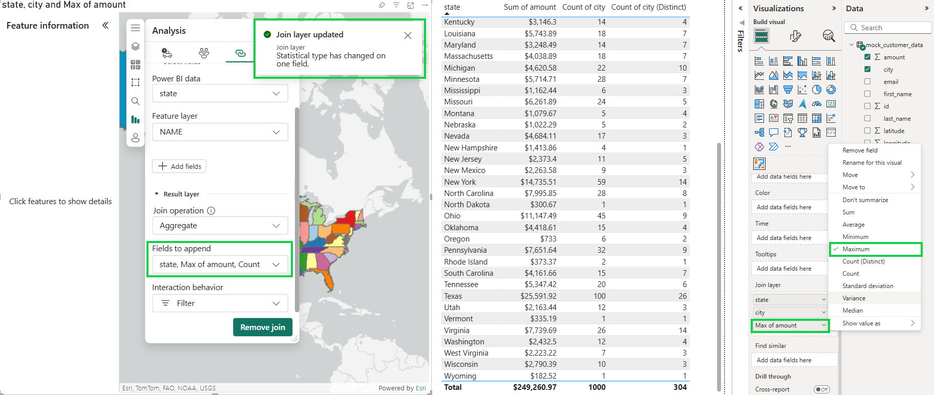
6. This statistical change (name and values) will be reflected in the Feature information pane as you select various features on the map.
7. Leaving the Join tool open, change the statistical type on amount to Standard Deviation.
   The join layer is updated, but notice that in Fields to append and in the Feature information pane, the field has been removed because Standard Deviation is not a supported statistical type when using join operation Aggregate.

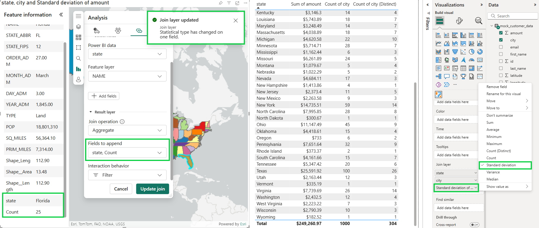
8. Close the Join layer tool and Join layer updated message.

Join operation change

Now see what happens to this join layer when you change the join operation type to Select first row only.

1. Remove and re-add the Sum of amount field to the Join layer field well.
   The Join layer field well should look like this:

2. Open the Join layer tool.
3. Switch the Join operation option to Select first row only.
4. Add all fields available in Fields to append. Notice that the Count field is no longer available when Select first row only is the join operation.

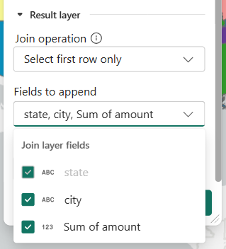
5. Click Update join to update the join layer.
6. Close the Join layer tool and the Join layer updated message.
7. Update the Table visual to show the state, city, and Sum of amount fields.
8. On the map, click the state of Texas again.
9. Scroll down in the Feature information pane.
   The last three fields are the fields in the join layer Fields to append section.
10. Notice in this example that the only city showing is Abilene, which is the first city in the Power BI data. Because you selected Select first row only as the join operation, only the first city record for each state feature is represented in the join layer data.

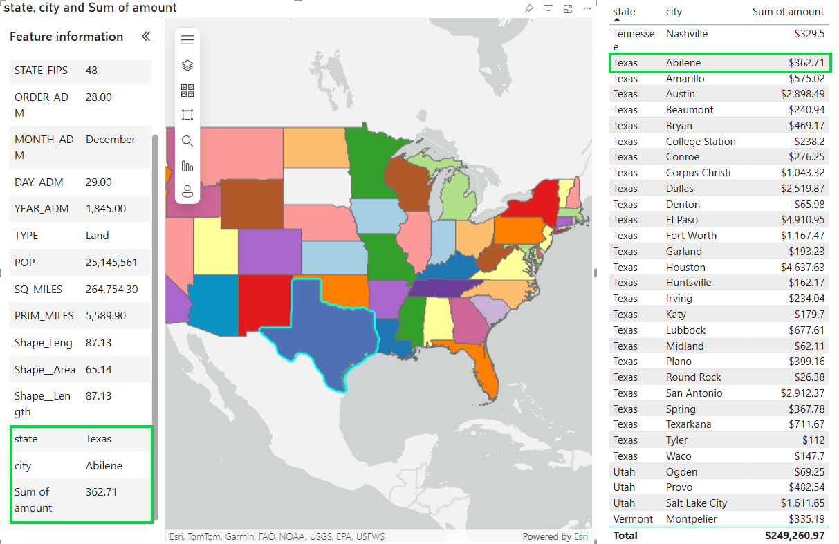
11. Open the Join layer tool.
12. Click the Join operation information button , and notice the cardinality is 1:n.

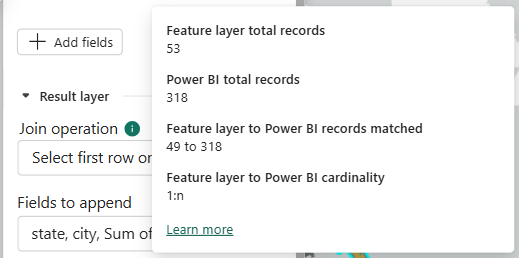
Explore unsupported statistical types

When the cardinality is 1:n, it is generally recommended that you choose Aggregate as the join operation. But when you choose Aggregate, some of Power BI’s statistical types aren’t supported in the join layer Fields to append fields. You can, however, make use of those statistical types. In this next example, you’ll make some adjustments to show just that. This requires switching the cardinality back to 1:1.

1. In the Join layer field well, add a second city field.
2. In the first city field, change its summarization to Count.
3. In the second city field, change its summarization to Count (distinct).
4. In addition, rename the second city field, adding (distinct) to clarify.

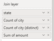
As you make this change, a Join layer updated message indicates an aggregation change.

5. Close this message.
6. Check the cardinality again.
   It is 1:1 because, apart from the state field, all other fields are summarized.

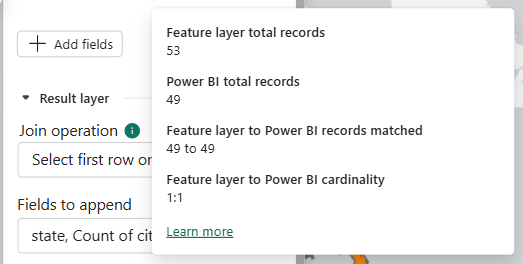
7. Update Fields to append to include all fields.

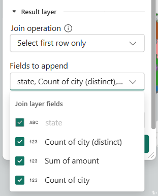
8. Click Update join.
9. Close the Join layer tool and Join layer updated message.
10. Update the Table visual to include comparable fields: state, Sum of amount, Count of city, Count of city (distinct).
11. On the map, click the state of Texas.
12. In the Feature information pane, scroll down to view the results.
13. View the Count of city (distinct) and Count of city fields to compare the unique city records per feature to the total city records per feature.

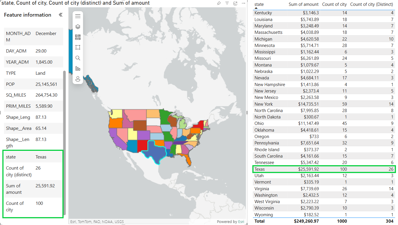
With this last example, you can see that even though the join layer Aggregate doesn’t allow some statistic types to be used in Fields to append fields, you can still use Power BI statistic types in specific cases as illustrated above, where the cardinality is 1:1 and the join operation is Select first row only.

Hopefully, these examples show why it is important to understand the nature of your data, your field well selections, how those selections affect cardinality and aggregation, and how your choices of Join operation and Fields to append affect the overall result of your join layer.

There are a wide range of possibilities in joining a single Power BI dataset with a single ArcGIS feature layer. Try different join layer examples with your data and available ArcGIS feature layers to gain a better understanding of how you can make use of this capability. Explore those examples alongside a Table visual of comparable fields to help guide your understanding of the data transformation and aggregation that occurs during the join process.

Appended join layer fields: Styling the joined result layer and labels

Styling the joined result layer is a new join layer feature of this release. You can change the visualization and legend of your new join layer using the fields belonging to the ArcGIS feature layer or Power BI data fields you add to the join layer using Fields to append.

Style the joined result layer

To style the joined result layer, complete the following steps:

1. Remove city fields from the Join layer field well.
2. Add the id field (don’t summarize) to the Join layer field well.
   Join layer fields include state, id, and Sum of amount.
   The id field ensures the highest granularity of the data, since id is the unique row identifier, Power BI will supply all rows of data in the dataset.

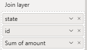
3. Before creating the join layer, lock the extent, if it’s not already locked. Zoom and pan the map to the U.S. contiguous states and turn on Lock extent in the Format Visual pane.
4. Collapse the Feature information pane on the map, if expanded.
5. Open the Join layer tool.
6. Click Remove join if join already exists.
7. Select US State Boundaries as the Target layer option.
8. For Power BI data, select field state and for Feature layer, select NAME.
9. For Join operation, select Aggregate.
10. Select all available fields in Fields to append (state, Sum of amount, Count).
11. For Interaction behavior, select Highlight.
12. Rename Result layer name to Join layer.

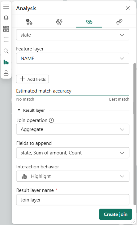
13. 13. Click Create join.
    14. Close the Join layer created message.
    15. Open the Layers pane.
    16. Click the Expand button to show the join layer’s legend.

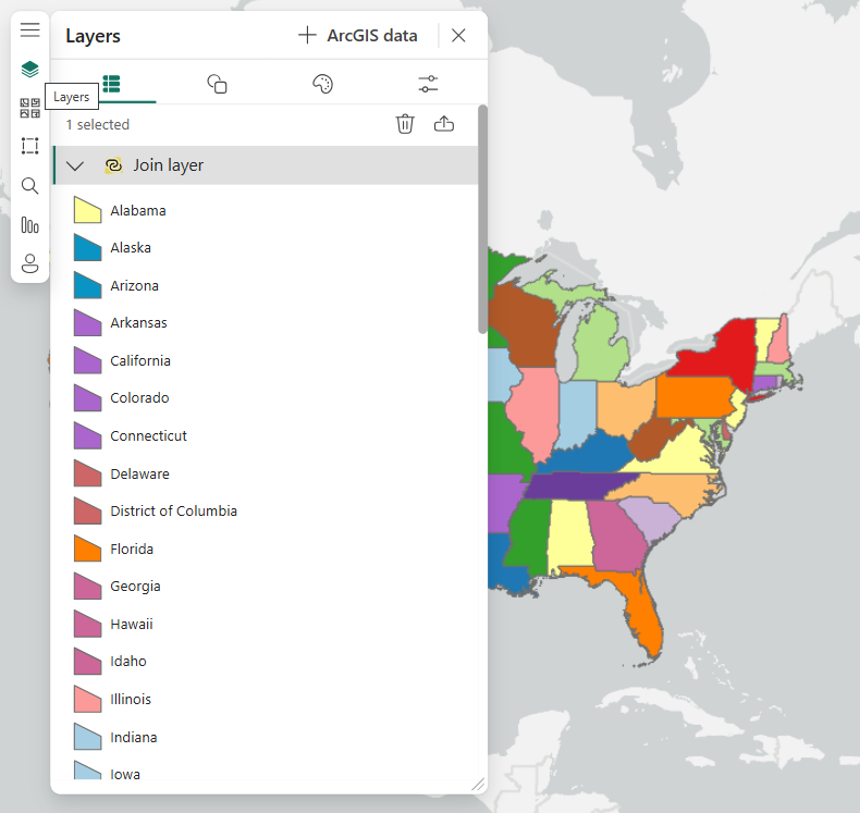
17. Click the Symbology tab.
    The default settings of the layer’s style show a Types visualization where each feature’s color is determined by the values in the NAME field as illustrated in the legend above.

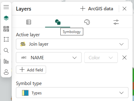
18. Click the field name drop-down menu and switch from the NAME field to the Sum of amount field.
    Each state is now rendered based on the Power BI data value Sum of amount for each state.

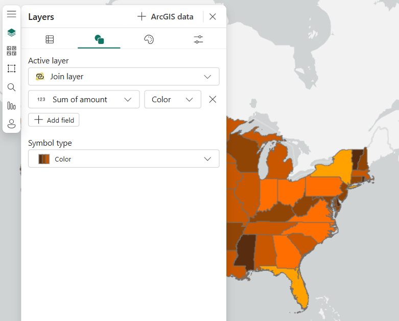
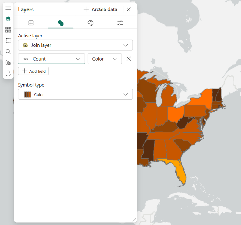
19. Click the field name drop-down menu, and switch from Sum of amount field to the Count field.
    There will be some subtle changes in color as each state is rendered based on the count of Power BI data records matching each feature (state).

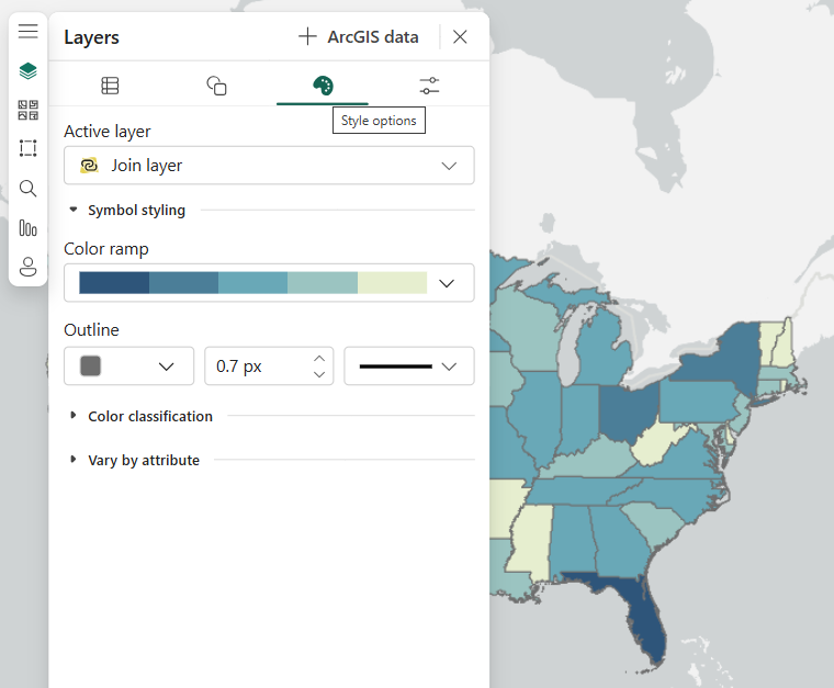
20. Click the Style options tab.
21. Under Color ramp, select Best for light backgrounds and select the Blue 2 option.
    
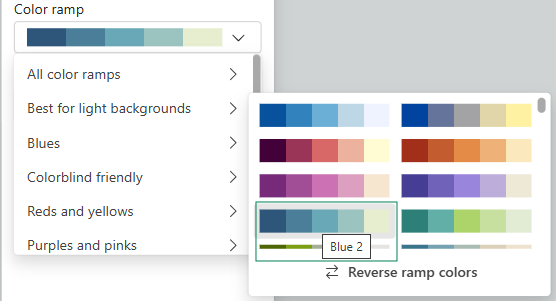
    The layer is rendered using the new color ramp.

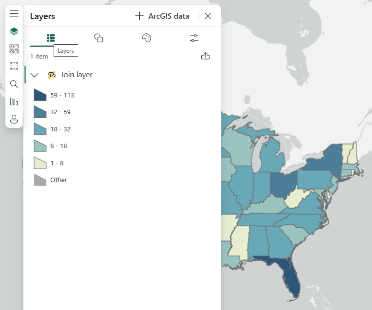
22. Click the Layers tab and view the updated legend.

Configure labels of the joined result layer

To configure labels of the joined result layer, complete the following steps:

1. Click the Layer properties tab.
2. Expand Labels.
3. Turn on Show labels.
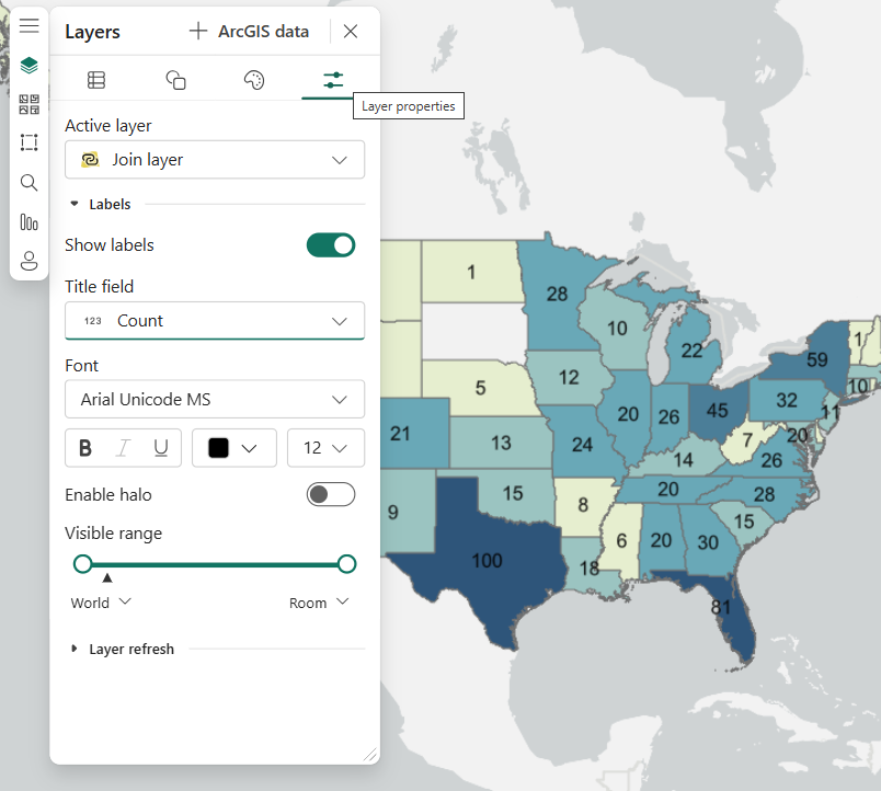
4. Switch Title field to show the join layer field Count.
   Each state now displays the count of Power BI records for each state corresponding to the values in the legend.

Style the joined result layer using multiple fields

To style the joined result layer using multiple fields, complete the following steps:

1. Return to the Symbology tab.
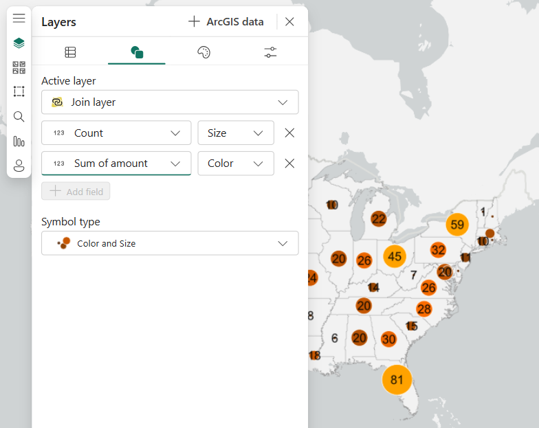
2. Switch Color to Size for Count.
3. Click Add field.
4. Select Sum of amount for the Color field.
   The feature layer symbol type changes and renders a centroid symbol illustrating relative counts and amounts by color and size.

Style a best practice choropleth map using the joined result layer

As mentioned above, when creating a choropleth map, it is best to use certain statistical values known as spatially intensive variables. In this example, you’ll use field Average of amount. In the following steps, you’ll adjust the current join layer, restore the Count label, and finally apply the style.

1. Close the Layers pane.
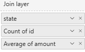
2. Change field id to Count of id in the Join layer field well.
3. Change field Sum of amount to Average of amount in the Join layer field well.

4. Close the Join layer updated message.
5. Open the Join layer tool.
6. Change the Join operation to Select first row only.
7. Open the Fields to append drop-down menu and select fields Average of amount and Count of Id.

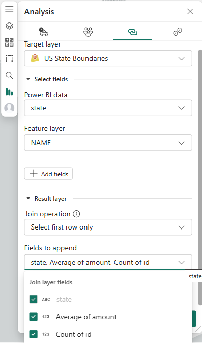
8. Click Update Join.
9. Close the Join layer updated message.
   Notice the Label field has been removed.

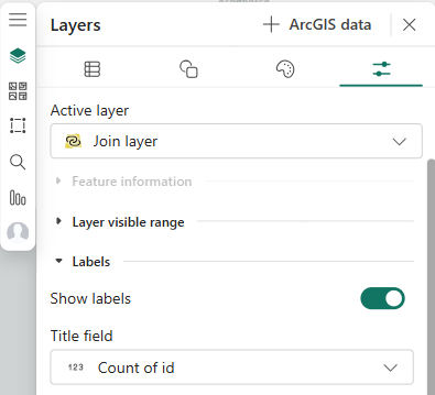
10. Open the Layers pane and select the Layer properties tab.
11. Click on Show labels.
12. Switch the Title field to join layer field Count of id.

13. Click the Symbology tab.
14. Click Add field.
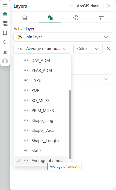
15. Switch Size to Color.
16. Select field Average of amount.

17. 17. Click the Style options tab.
    18. Under Color ramp, select Best for light backgrounds and select the Blue 2 option.
        
        The layer is rendered using the new color ramp.
    19. Click the Layers tab.
    20. Click the Expand button to show the join layer’s legend.
        The choropleth map is using statistic Average of amount for the theme and Count of id as the label.

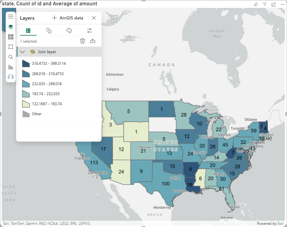
This is only an introduction to what you can do using styling and labeling. Explore the many options available. You can read further about Layer styling in ArcGIS for Power BI.

Join layer and related feature layer on the map

In the examples above, you didn’t create a feature layer in the map prior to creating the join layer. While that used to be a requirement for creating a join layer in previous releases, it is no longer necessary.

Create a join layer targeting an ArcGIS feature layer already on the map

Next, you’ll learn about the distinct behavior of a feature layer added to the map prior to join layer creation and how these layers interact.

1. Create a new report page using the same mock customer data file used earlier.
2. Add the ArcGIS for Power BI visual to the blank report page.
3. Sign in to ArcGIS or continue as a guest.
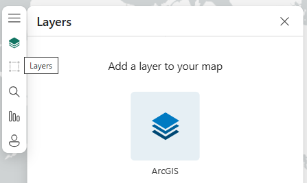
4. Open the Layers pane.
5. Click the ArcGIS button.

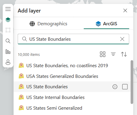
6. Search for and add the US State Boundaries layer and click the check box to add the layer.
   Note: If you signed in, ensure you are searching in the ArcGIS Online category.

7. After adding the ArcGIS feature layer, click Done.
8. Open the layer’s More options menu on the right and click the Create join layer button.

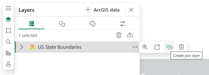
The Join layer tool is opened, but no join layer fields exist yet.

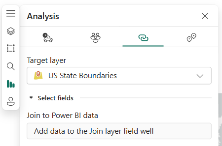
9. Drag state and amount into the Join layer field well.
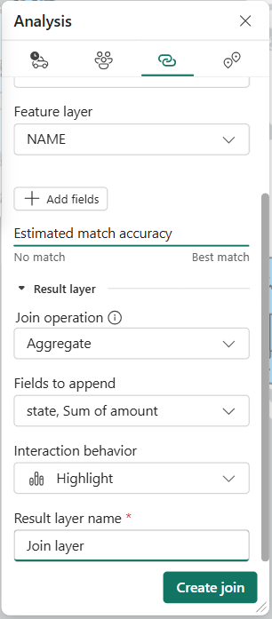
10. Select state and NAME to define the join under Select fields.
11. For Join operation, select Aggregate.
12. For Fields to append, select state and Sum of amount.
13. For Interaction behavior, select Highlight.
14. For Result layer name, type Join layer.
15. Click Create Join.

The join layer is created, and the message confirms the feature layer has been hidden.

16. Close the Join layer tool.
17. Pan and zoom the map so you can see the 48 contiguous U.S. states.
18. Open the Layers pane.
    The join layer and the feature layer are shown, but the feature layer is hidden.
    Note: The join layer represents all the states in the Power BI data, and two states are missing: Maine and South Dakota.

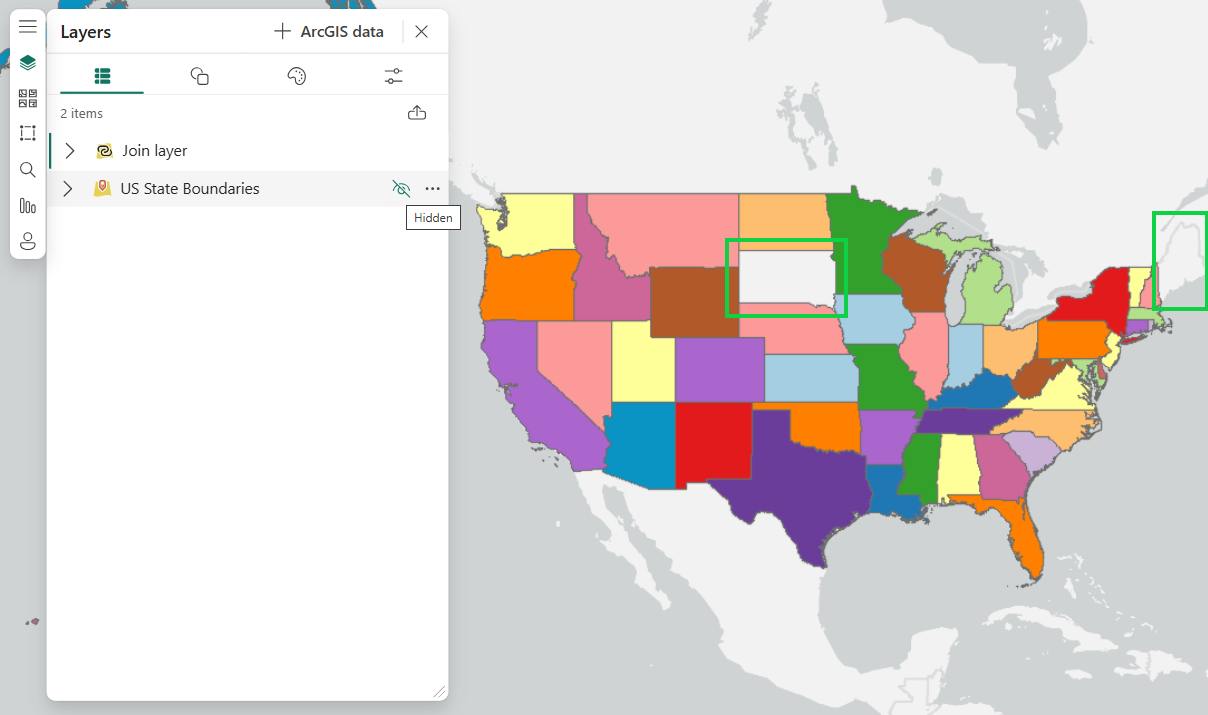
19. Click the Hidden button on the US State Boundaries layer to make it visible.
20. Notice that when the US State Boundaries layer is made visible, the South Dakota and Maine state features appear.

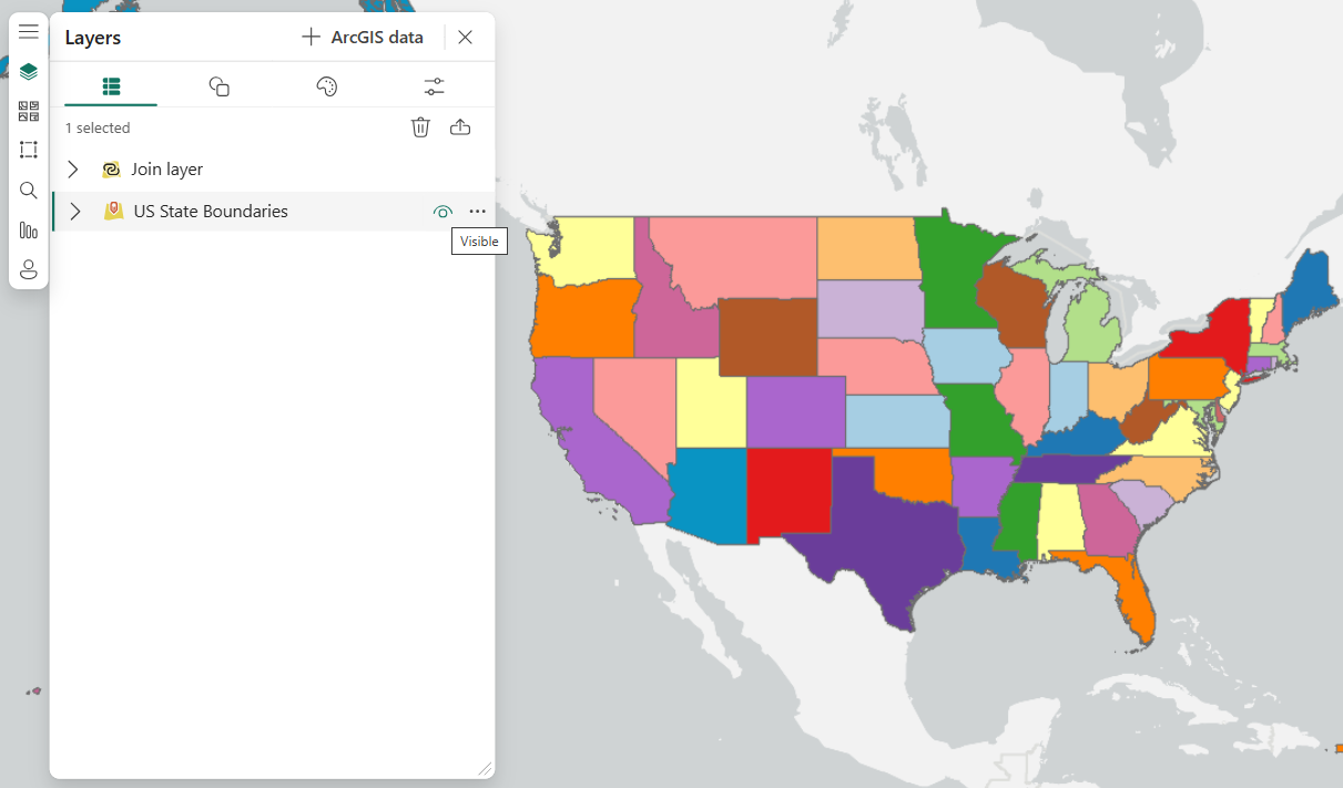
When created, a join layer is placed on top of the ArcGIS feature layer to which it is joined. But when both are visible and both have the same style, it obscures the nature of the join. In this example, you no longer see the missing features represented by the join layer. This is why the ArcGIS feature layer is hidden automatically once the join layer is created.

Change the styling of the joined result layer and added feature layer

You can choose to show or hide the feature layer after creating the join layer, but keep in mind how it may obscure the join layer when they have the same style. For the next example, you’ll keep both layers visible and change their styles.

Note: Styling feature layers that contain Arcade expressions is not supported.

21. Temporarily hide the join layer and show the feature layer (US State Boundaries).
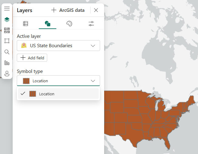
22. Click the feature layer and select the Symbology tab.
23. Switch Symbol type to Location.

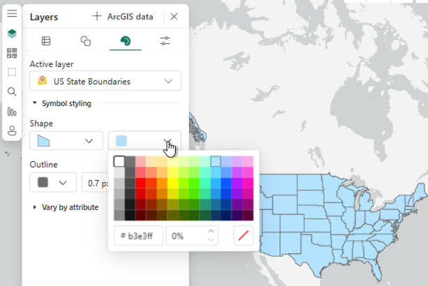
24. Select the Style options tab and change the fill color to a light blue.
    The color should contrast with the color scheme of the join layer.

25. Click the Layers tab, select the join layer, and make it visible again.
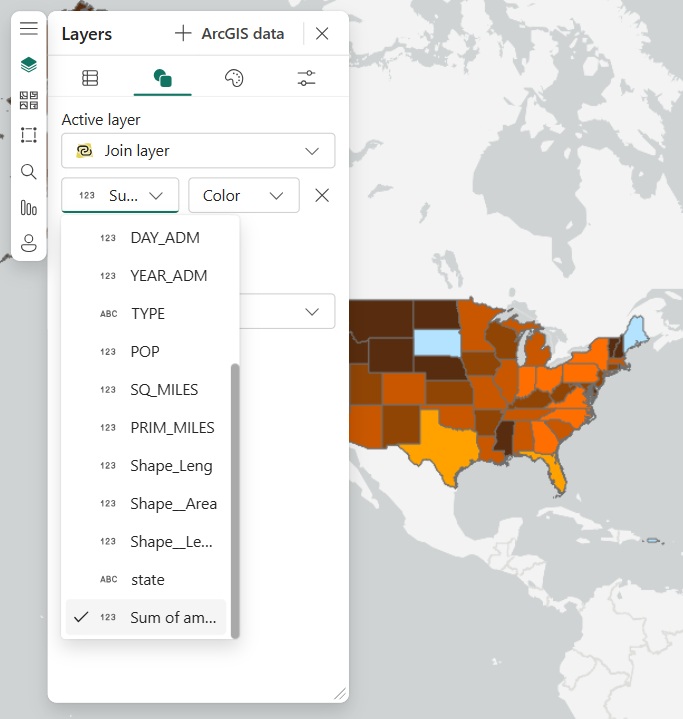
26. Click the Symbology tab and switch the field to the Power BI data field Sum of amount.
27. With contrasting styles, leave both layers visible.

28. Create a Power BI Table visual using fields state and Sum of amount.
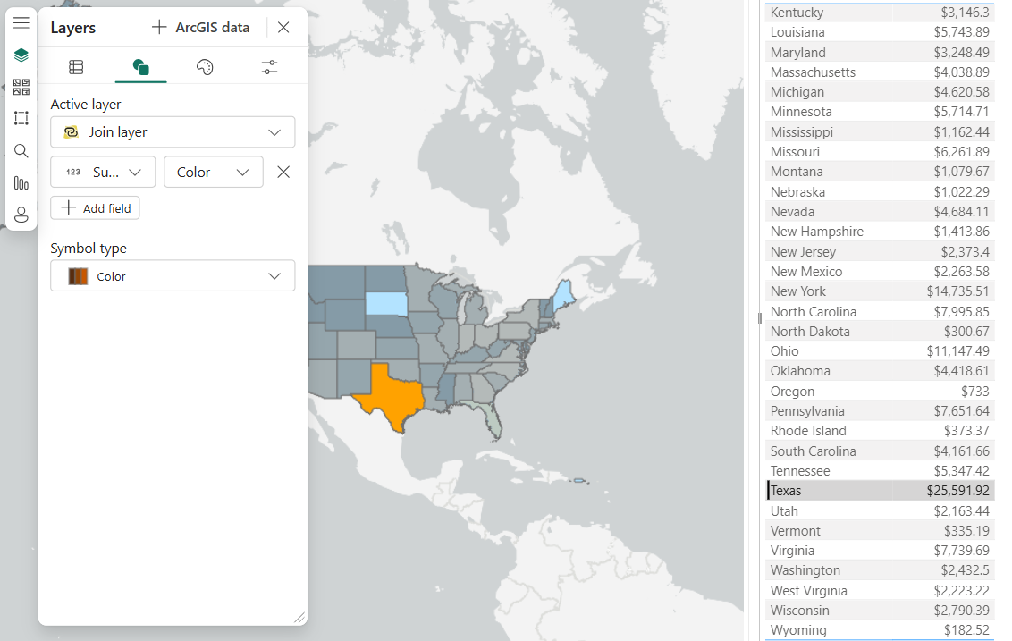
29. Select the state of Texas in the Table visual.
    Here you can see the benefit of contrasting styles.
    There are three categories of features: the selected feature (Texas), unselected features (other states), and features not included in the join (South Dakota and Maine).

You can now understand and use the new join layer features to visualize Power BI data in meaningful and effective ways.

Recommendations

The following are key recommendations when using the join layer feature in ArcGIS for Power BI:

• For best results, use matching unique key values when you select fields in the Join layer tool in both the ArcGIS feature layer and the Power BI data.
• When choosing the key fields of the join, consider if these key fields are geographically relevant. This will lead to better results.
  • Do the key fields themselves represent a specific geographic location or feature (for example, country, state, region, city, or zip code)?
  • Do the key fields (for example, assetID field, where the asset has a location) relate to unique rows in the feature layer, which themselves represent a geographic location?
• When creating a join layer or checking the cardinality of a join layer, it is recommended that you remove data filters—for example, temporary selections or filters in other visuals, slicers, or page and report filters.
• Use the Select first row only join operation when the join cardinality is 1:1; otherwise, results are truncated.
• Use the Aggregate join operation when the join cardinality is 1:n or n:n.
• Layer creation order is important. If using both a Power BI data layer and a join layer on the same map, create and modify the data layer first and then add the fields necessary for the join only in the Join layer field well before creating the join layer.

Caveats

The following are caveats when using the join layer feature in ArcGIS for Power BI:

• The fields in the Fields to append drop-down menu can use fields added to any field well.
  • Recommendation: It’s best to use only fields that have been added to the Join layer field well.
• Removing and adding fields to any field well after the join layer is created can cause aggregation changes in the join layer, as illustrated in the Explore aggregation section above.
  • Recommendation: Know your data and be aware of aggregation changes that are a result of adding and removing fields from field wells. If possible, add all needed fields to field wells prior to creating the join.
• Join layers can be created when page or report filters and slicers are applied. There will be a warning when this occurs. This will create a join that is only a subset of the features available.
  • Recommendation: This may be the intended use of the join layer, so it’s allowed. Be aware of the impact of applying these kinds of data filters both before and after the join layer is created.