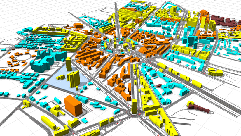
In the image below, you can see buildings of various sizes. Additionally, you can see a variety of tree canopy sizes, road orientations, and ship lengths.

Accurately extracting features from satellite and aerial imagery can come with many challenges, such as multi-sensor data and variability in object sizes, scales, and spatial resolutions. A single image, like the one above, can contain various information, each requiring precise segmentation. Additionally, if you are familiar with deep learning feature extraction workflows, you know that a deliberate quality assurance and quality control (QA/QC) process is required to obtain the best and most accurate results.

To address the challenges posed by the diversity in input datasets and expose deep learning models to all possible variations during training and inference, you can employ techniques like data augmentation and test-time augmentation.

Data augmentation

Data augmentation is a technique for artificially expanding the size and diversity of a training dataset by applying various transformations to the existing training data. It enhances the model’s ability to generalize effectively during training, leading to improved performance in real-world scenarios. Some commonly used data augmentation techniques include image rotation, horizontal and vertical flips, and changes in scale, brightness, and contrast.

Test time augmentation

Test Time Augmentation (TTA) is a powerful experimental technique that applies data augmentation to the input image during the testing or inference phase and averages the predictions from the augmented versions to enhance output accuracy. It improves a model’s generalization ability by exposing it to a wider range of input variations during inference. The final output is more reliable because it synthesizes insights from multiple perspectives of the same input data. The general process of TTA during inference is as follows:

1. Augment the input image—The input imagery is transformed using predefined augmentations such as rotation and flipping.
2. Generate predictions—The model generates predictions for each augmented version of the input.
3. Aggregate results—Predictions from all augmented versions are combined using aggregation methods such as averaging or weighted averaging.

ArcGIS Pro supports dihedral transformations (D8) during inference. The D8 transformation transforms the test image in eight dihedral angles if map space is used and in two dihedral angles (original and flipping horizontally) if pixel space is used. Let’s understand these dihedral angles.

D8 is an all-square-symmetry group, which includes anticlockwise rotations by 0, 90, 180, and 270 degrees and reflections across the horizontal, vertical, and two diagonal axes, as shown below.

The image below shows how satellite imagery transforms by applying these dihedral transformations.

Next, let’s visualize the impact of these transformations on inferencing.

You can observe the difference in the output quality of segmented roads with and without utilizing the TTA technique.

You can apply test time augmentation in ArcGIS Pro using the Detect Objects Using Deep Learning tool, the Classify Pixels Using Deep Learning tool, or the Classify Objects Using Deep Learning tool. If the ‘Test Time Augmentation’ model argument is set to true, predictions of flipped and rotated orientations of the input image will be merged into the final output, and their confidence values will be averaged. This may cause the confidence values to fall below the threshold for objects detected only in a few orientations (of the image). The ‘Merge Policy’ argument applies to merging augmented predictions using mean, max, and min algorithms. It is only applicable when TTA is used.

Multi-scale test time augmentation

Among the various transformations used in TTA, changing the scale of the input image has proven to significantly improve results for geospatial use cases. This is because features in satellite or aerial imagery appear at different scales. For example, small objects like cars or trees are easier to detect at higher resolutions (e.g., 5 cm), while larger objects like buildings or ships are easier to detect at relatively coarser resolutions (e.g., 30 cm or 40 cm per pixel).

Multi-scale test time augmentation is an augmentation technique used to improve the performance of deep learning models, particularly for tasks such as object detection, during the testing phase. With this technique, the input image is resized to different resolutions or scales, and the deep learning model is made to run on each version. The results from these multiple scales are then combined, typically by weighted averaging, to produce a more accurate and stronger final prediction. Multi-scale TTA allows a single deep learning model to adapt to multiple resolutions and reduce scale bias.

Multi-scale TTA and multi-resolution adaptation

By using the ‘tta_scales’ model argument during inference, the input imagery is resampled to multiple resolutions during inference, and the model processes the same image at various resolutions. For example, let’s assume that the original cell size is 30 cm; if we provide different scales in the ‘tta_scales‘ model argument, it means:

• At scale 0.5—upscaling the imagery to a higher resolution (in this case, from 30 cm to 15 cm). This makes smaller objects like tree canopies or vehicles more discernible to the model.
• At scale 1.0—using the original resolution (i.e., 30 cm). This ensures consistency with the model’s training data and original input resolution, which often provides the baseline for accurate predictions.
• At scale 1.5—downsampling the imagery to a coarser resolution (in this case, from 30 cm to 45 cm). This makes larger objects like buildings or ships become more prominent, and noise from finer details is reduced.

Other scales, such as 0.2, 0.9, 1.2, and 2.0, can also be tried. Different combinations of scales work better for different features.

Multi-scale TTA enables the model to detect objects of varying sizes by more effectively resampling the image to different resolutions, producing more generalized and reliable outputs. If various objects are provided in a single text prompt to the model, the model can detect multiple multi-scale features from the same imagery in a single run. For example, if you provide “cars, trucks, and ships” as the text prompt, the model will try to detect all of them in the provided input imagery.

Multi-scale TTA and reduction in scale bias

A model trained at a specific resolution often develops a bias towards detecting objects at that resolution. For example, a model trained at 50 cm resolution might miss smaller objects if applied to higher-resolution data (e.g., 10 cm), as these objects may not have been adequately represented in the training dataset. Retraining a model for each scale can be time-consuming and computationally expensive. TTA scales mitigate this bias by exposing the model to multiple resolutions during inference. By aggregating predictions across the scales, the final output becomes resolution-independent to an extent, significantly improving the model’s performance.

Benefits of multi-scale TTA

• By widening the perspectives, the model improves its ability to detect objects and becomes effective at dealing with resolution variability. It aims to detect small, medium, and large objects in a single workflow.
• Multi-scale predictions try to ensure that no object is missed, regardless of size.
• Handles input imagery of different resolution than the training data resolution.
• A single model can be used to detect different-scale features simultaneously from the same scene.
• Small objects become more apparent in high-resolution upscaled imagery.
• Large objects are easily captured in downscaled imagery.
• The argument reduces scale bias.

Multi-scale TTA can be applied in object detection tasks after training a model using the Train Deep Learning Model tool and using the saved model for inference using the Detect Objects Using Deep Learning tool.

Let’s see how we can apply multi-scale TTA in the Text SAM pretrained model in ArcGIS Pro.

Multi-scale TTA in Text SAM model

Text SAM is a powerful open-source AI model that can be prompted using free-form text prompts to extract various features directly from imagery. It achieves this using two state-of-the-art AI models—Grounding DINO and Segment Anything Model (SAM)—without requiring predefined classes. The features, which are described by the input text prompts, can be any object of interest, such as vehicles, swimming pools, ships, airplanes, solar panels, and so on.

Unlike traditional detection models trained on fixed classes (for example, cars, solar panels, and trees), TextSAM can detect any object described in the text prompt, making it highly versatile. With this model, users don’t need extensive training data or technical expertise to extract features. The text-prompt-driven approach makes it intuitive and accessible. However, what makes TextSAM even more effective in real-world applications is its ability to handle multi-scale features in a single scene. It allows the model to adapt to varying scales during inference, ensuring accurate and higher confidence results even when the imagery resolution doesn’t match the training data.

We will now explore how multi-scale TTA enhances the performance of the TextSAM model, enabling it to detect objects of varying sizes. Let’s dive deeper into how it works and why it matters.

Use multi-scale TTA in ArcGIS Pro

The figure below shows how we can provide different combinations of scales in the ‘tta_scales’ argument of the Text SAM model.

We experimented on an image containing swimming pools with and without implementing ‘tta_scales’. The results show that the model could not detect a few swimming pools when ‘tta_scales’ was not utilized.

For more information on how to use the model, see the ArcGIS pretrained models documentation or TextSAM learn lesson.

Comparison of outputs with and without multi-scale TTA

Practical tips for using multi-scale TTA effectively

While multi-scale TTA can significantly enhance the performance of models, applying this technique effectively requires thoughtful planning and consideration. Here are some practical tips on how to optimize the use of ‘tta_scales’ for geospatial workflows:

• Choose the right scales based on objectives—the choice of scales should align with the type of object you want to detect and the resolution of your input imagery. Consider the following:
  • Start with the scale corresponding to the model’s training resolution.
  • For small objects, add smaller scales (for example, 0.5) to upsample the imagery and make fine details like vehicles, small tree canopies, and narrow roads more visible to the model.
  • For medium-sized objects, retain the original scale (1.0) to maintain consistency with the model’s training resolution, which is often designed to capture objects of average size.
  • For large objects, add larger scales (for example, 1.5 or 2.0) to downsample the imagery and emphasize more prominent features, such as buildings, industrial zones, or large ships.
  • Experiment with a range of scales (for example, [0.5, 1.0, 1.5]) to capture a broad spectrum of object sizes within a scene.
  • Pay attention to patterns, such as specific scales performing better for certain object types or imagery sources. Conduct validation with ‘tta_scales’.
• Balance between scale range and computational resources—Applying too many scales during inference can be computationally expensive and time-consuming. For example, while inferencing over the same area using inputs of 1 and 0.5, 1, and 1.5 for the tta_scales argument, the tool took 43 seconds and 2 minutes and 50 seconds, respectively, to complete the processes when other settings weren’t changed.

To strike a balance:

• • Limit the number of scales to a manageable range (for example, 2-3 scales) based on the complexity of the dataset and the available computing power.
  • Prioritize scales that are most likely to improve performance based on the resolution of the input imagery. For example, if the input imagery is at 50 cm, start with [0.75, 1.0] to focus on small and medium objects.
  • Using a few but well-chosen scales can save resources while still delivering significant improvements in accuracy.
  • Use GPUs or high-performance computing clusters for faster inference.
  • Downsample large datasets during experimentation to test scales efficiently and identify the most effective configuration before applying it to the entire dataset.
• Understand the trade-offs between precision and speed— While multi-scale TTA improves accuracy, it also introduces additional processing time due to multiple passes through the model. Consider these trade-offs:
  • When accuracy is critical, for tasks like disaster response, environmental monitoring, or precision agriculture, the slight increase in processing time is justified by the improved detection quality.
  • When speed is essential for time-sensitive applications, such as real-time traffic analysis, limit the number of scales to ensure faster results while maintaining reasonable accuracy.
  • Evaluate the specific requirements of your project to determine the appropriate balance.
• Customize for your geospatial application—Different geospatial tasks require different scale combinations and strategies. Some examples include
  • Urban planning—Use scales like [1.0, 1.5] to capture buildings of different sizes.
  • Maritime applications—Incorporate [1.0, 1.5, 2.0] scales to detect ships of different sizes in high-resolution imagery.
• Monitor the quality of results—Despite its benefits, multi-scale TTA isn’t foolproof. Quality assurance and quality control (QA/QC) checks are essential to ensure the model performs as expected:
  • Ensure that the final output aligns with ground truth data or expert validation.
  • Verify that smaller scales do not introduce noise or false positives in the output.
  • Ensure larger scales do not oversimplify detection boundaries.

Limitations of multi-scale TTA

A model trained at a specific resolution may struggle with extreme upscaling or downscaling.

We must be careful when choosing the right scale. Extreme scaling led to the detection of green cover as trees.

• For datasets where all objects are roughly the same size, scaling may add unnecessary complexity.
• Large differences in resolution between training and input data might introduce artifacts or lead to the loss of meaningful spatial features.
• Running inference at multiple scales increases computational load and memory requirements. The inference time is directly proportional to the number of scales used.
• Overlapping information across similar scales can lead to redundancy, which might not significantly improve results. Without proportional gains, additional computational cost becomes less justifiable.
• In cases where the data is already in low resolution, scaling down further can degrade feature visibility.
• Different scales may lead to slight misalignments in predictions, requiring additional post-processing for consistent results.
• Manual selection of scale values. Identifying optimal scales requires trial-and-error, which can be time-consuming. Poorly chosen scales might not align with the feature sizes in the dataset, leading to little or no improvement.
• If the model is trained on low-quality or imbalanced datasets, multi-scale TTA may have limited impact. If the model architecture is not strong, scales cannot fix fundamental flaws in feature extraction. A poorly trained model will still produce inaccurate predictions at multiple scales. Multi-scale TTA cannot create information that the model has not learned.
• Higher energy consumption contributes to a larger carbon footprint, a growing concern in AI practices.

Here are some more outputs:

Test time augmentation has conclusively proven to be a powerful technique for improving the accuracy and strength of deep learning models in geospatial analysis. Using dihedral transformations and multiple scales input during inferencing allows models to better handle variations in object sizes, resolution differences, data heterogeneity, and complex geographic features. This approach significantly enhances model generalization and boosts performance across diverse datasets and applications in industries ranging from urban planning to environmental monitoring to maritime planning. However, the journey doesn’t end here. While TTA and Multi-scale TTA offer significant benefits, their effective implementation requires careful consideration of computational costs, scale selection, and domain-specific requirements.

At the heart of this approach lies a simple but profound idea: looking at the world from multiple perspectives, we gain a deeper understanding of its complexity. This is what TTA enables: a more nuanced and informed view of geospatial data, empowering better decision-making across industries. Whether you are a researcher, data scientist, or geospatial professional, embracing techniques like Multi-scale TTA and carefully balancing their benefits and limitations can help you push the boundaries of what’s possible.

We are excited to see how you apply these insights to your own geospatial workflows and drive innovation in the geospatial field. Whether you are a seasoned professional or just starting to explore the world of geospatial AI, the potential to innovate is at your fingertips.