With the June 2020 release, ArcGIS Online provides layer blending in Map Viewer Beta. Mark Harrower has this great introduction to blend modes here, which goes over four of his favorite uses of them. In this blog, I focus on blend modes that improve your thematic maps, especially for maps of polygon layers.
In summary, a blend mode takes two or more layers, and “blends” the pixels normally drawn by each layer, based on the rules inherent to each blend mode. There are more than 30 blends modes available in ArcGIS Online. There are infinite combinations of layers, subjects, use cases etc — too numerous to stuff into any one blog. I chose a few of the more eye-catching blend modes to highlight in this blog.
Top Down Map Drawing
One of the first things you learn when making maps is how to place one layer on top of another, in a vertical stack, so that the topmost layer draws on top of all the layers underneath it. We learn to put polygons on the bottom, then lines, and finally points on top.
Whatever layer’s features are on top get drawn last, and everything underneath those features are blocked from being seen. It’s a “winner take all” game for each pixel on the map.

Fortunately, we have two other options when drawing things on the map: transparency and blending. You’ve probably used transparency before but may not have thought about using blend modes on your thematic maps. Let’s compare the two approaches.
Benefits and Limits of Transparency
Transparency is one way you can mix two or more layers’ information. For example, you can set a polygon layer’s transparency to 50% transparent so that the basemap’s features can also be faintly visible. In the map below, the yellow service areas are within 11 minutes of a hospital emergency room. I set the yellow polygons to be 50% transparent so that some of the basemap’s content would show through.
The undesired effect was that the entire map gets “softer” visually, and the labels and features struggle to show underneath the polygons. It doesn’t look crisp. It doesn’t look as professional as you might desire. It’s not bad, but it isn’t great. Why? The labels are not as crisp as the basemap author intended, and the yellow polygons, red lines and blue hospitals are likewise not as crisp as the layer author intended. So, it works, but it’s not great:

The issue is more evident when mapping a layer of polygons on top of a basemap. The polygon layer of median household income covers up 100% of the basemap’s labels, roads, and mountains. So I added 30% transparency to the polygon layer, and put the roads on top and set them 30% transparent. As a consequence, everything on the map is washed out in terms of color by the use of transparency:

About 10 years ago, Esri expanded the definition of an online basemap to include a “base” layer and a “reference” layer to help you improve your thematic mapping. A base layer is one that always draws on the bottom of the stack of layers, while a reference layer always draws on top of everything else in the map. Think of it as a “map sandwich” where the base and reference layers are the bread, and you choose which layers to put in between. Note how the labels are much more clear in the example below.

This reference layer also allows us to turn off transparency on the polygons layer. As a result, its colors are much more vibrant and help the map clarify its subject (median household income):

While this thematic map now has a cleaner look, the solid blocks of color that the polygon layer brings to the map cover up all the underlying basemap information. Even with transparency turned on in the above examples, you don’t really see how the physical structure to the land is affecting the map’s subject. What if you could use the full color palette in your maps AND have useful information from the basemap show through as well?
Blend: Transparency’s Better-Looking, More Talented Sibling
Software programs like Photoshop have had a “blend” capability, where the software performs calculations on each layer’s pixels to apply various visual effects to those pixels. In the example below, geology polygons plus terrain equals a much more pleasing map because the terrain has something to do with the polygons’ topic.

This version of the income map blends the polygon layer’s colors with a layer containing elevation data, expressed as a hillshade. You’ve probably seen maps like this in textbooks and other print maps before. They are now easily configured in an online map as well.

A couple of blend modes stood out to me with regard to their use in thematic maps like the examples below.
Multiply example
To keep things simple in the examples below, we blend the topmost layer in the web map with the layers underneath it. The technique is pretty simple. Add the layers to your web map, choose the topmost layer, and set its blend mode under that topmost layer’s Properties.
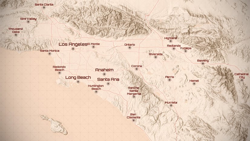
The multiply option is excellent for blending mountain ranges with polygons. In the past, if you wanted to see mountain ranges with color on top of them, you would apply transparency of 30% or more, making the colors wash out for the most part. With multiply blend mode, there is no need to use transparency, as the mountain hillshading is blended into the colors. This web map begins to look like the maps you see in textbooks:

Destination-atop example
The destination-atop mode is excellent for blending patterns of land use, population grids, and business locations with polygon choropleth maps of statistical data or polygon choropleth maps of categories. Rather than fill an entire polygon with color, try destination-atop blend to color only those areas within the polygon that are actually related to the map’s subject. In the example below, WorldPop’s Populated Footprint in 2020 layer available in ArcGIS Living Atlas is blended with a diversity index by census tract layer. Instead of a continuous surface across the country, we see the settlement patterns emerge within the ZIP Codes data.


In the web map below (login required), looking at diversity northwest of Berkeley, CA, we see that populated areas fill with color, while areas that are sparsely populated or empty get no color. More diverse areas are shown in red, less diverse areas are shown in blue. The basemap’s information helps explain why an area appears to have no data – it is because that area is not populated. This example uses destination-atop mode on the population layer, and puts the layers into a group, then applies the multiply mode to the group layer.

In the map below of diversity index around the Front Range, Colorado, the destination-atop blend mode gives a more accurate depiction of how we live than solid blocks of color, which imply a continuous pattern across the land. This map reveals the density of the subject. Solid color blocks of polygons hide it.

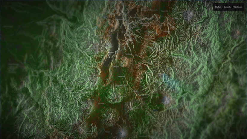
In the next example web map below (login required), we see Global COVID-19 Trends by country from ArcGIS Living Atlas, blended with WorldPop’s Populated Footprint in 2020 layer available in ArcGIS Living Atlas. Densely populated countries become more self-evident in this view. Purple areas are in Epidemic or Spreading stages. Norway’s coastal population is in evidence, as are densely populated India and Ireland. Can you spot Cairo, Egypt and the Nile River?

This view below of Indianapolis does a good job depicting COVID-19 Trends by County information within the densely populated downtown, as well as suburban areas and smaller towns surrounding the city. At the time this image was taken, downtown was in Epidemic stage, while the county just north is in Spreading stage.

In the map of air quality below, the hexbin polygons of PM 2.5 measures are visually blended with a layer of business locations to visualize these related topics (example web map)

In this example, the predominant crop in each county is blended with the NLCD land use data for cropland. Each pixel that is known to be working cropland is shaded according to what the predominant crop in the county happens to be. Corn (yellow), soy (blue) and wheat (green) to reveal these summary statistics through the lens of the land which support them.

This type of combination can work with many other pairs of layers: blend population grids with any demographic or statistical analysis results; business locations with sales or market opportunity; residential land use with tax revenues by county… it is a different way of thinking about your layers blended with other layers.
Log in to ArcGIS Online, add some layers to Map Viewer Beta, choose the topmost layer and cycle through each blend mode to see what it does. I highly recommend you take 15 minutes of your day to try that out. After doing that, try out Multiply mode and Destination-atop mode in the Map Viewer Beta. What other combinations of thematic content and blend modes are you thinking about? As always, thoughts and feedback are welcome in the ArcGIS Online Ideas community site.
All images by Jim Herries unless otherwise noted.


Article Discussion: