For the past 50 years, Landsat satellites have produced a lot of image data, and the new Landsat 9 will add even more to the archive. The longest continuous time series image data has provided us with opportunities to study land-cover change in any location on our planet.
The Amazon floodplains are some of the most valuable ecosystems on earth, hosting an environment suitable for both aquatic and terrestrial life forms. The seasonal land cover alternation due to the seasonal floods establishes a harmony for the life forms in this unique ecosystem. We want to investigate and identify permanent changes to the floodplain forests that may alter the ecosystem and affect wildlife habitats. To find the answer, we will analyze the Landsat time series data using the LandTrendr change detection capabilities in ArcGIS, processing the data using ArcGIS Notebooks with the ArcPy image analysis module and display the analysis results using advanced visualization capability in ArcGIS Pro.
Study area
The study area is in the lower Amazon floodplain covered by Landsat scenes identified with path=228 and row=061, shown as a yellow box in the picture below. The images are surface reflectance products from Landsat Collection 2, recommended for image time series analysis. The images taken during September and October are better suited for our study as these are the months when floods retreat, and land covers emerge. We selected all possible images within these two months from 1984 to 2021 with cloud cover of less than 10 percent.

Workflow
ArcGIS provides capabilities to analyze change in many ways: compare two images using the Change Detection Wizard, detect change time points from an image time series using the Continuous Change Detection and Classification (CCDC) or LandTrendr algorithm, or simply visualize change by composing multitemporal images as a multiband and displaying images using the RGB renderer. In this study, we will use the LandTrendr change detection tool.
LandTrendr (Landsat-Based Detection of Trends in Disturbance and Recovery) is an algorithm proposed by Kennedy et al. and supported in ArcGIS. For an image time series, the LandTrendr algorithm analyzes each pixel’s trajectory along a timeline using linear regression. The resultant regression model is a set of segments that characterize the change events, such as change start and end dates, within how many years did the change occur, and what the change magnitude is. In ArcGIS Pro, this algorithm is supported by two geoprocessing tools: Analyze Change Using LandTrendr and Detect Change From Change Analysis Raster tools. (Note: If you plan to use ArcGIS Enterprise or ArcGIS Online, LandTrendr change detection capabilities are available as raster functions in ArcGIS API for Python. See the Change detection of time series imagery blog for an example of processing using ArcGIS Enterprise.) Below is the workflow of image time series change detection used in this blog.

1. Create an image cube
There are a few ways to prepare data for image time series analysis: create a raster collection object directly from a folder of source images; create a mosaic dataset; or create a multidimensional Cloud Raster Format (CRF), which is called an image cube. We chose to create a multidimensional CRF as it is optimized for time series analysis. We used the steps documented in this blog and created an analysis-ready image cube stored in a multidimensional CRF. To start the process, we will import the arcpy.ia image analysis module, check out the ArcGIS Image Analyst license, and then create a multidimensional raster object from the CRF.

Next, we will create a Normalized Difference Vegetation Index (NDVI) image cube since our goal is to analyze land-cover change in the Amazon floodplains, and NDVI is effective in separating water from vegetation or nonwater land cover. The code below simply uses an NDVI function to create the NDVI image cube and displays the most recent slice of the NDVI. Water has negative NDVI values and is rendered in pink.


2. Create a change analysis raster
In this step, we want to analyze the NDVI image cube using the Analyze Change Using LandTrendr tool. The tool has many parameters, but we can simply use default values because these are already optimized for Landsat images.

The process generates a change analysis raster, which is a multidimensional raster that contains one raster for each year, and each raster is multiband where bands are the regression coefficients. Below is the RGB display of the change analysis raster where the red band is the slope, the green band is a fitted NDVI value, and the blue band is the change magnitude. Yellow-green represents vegetation, and dark pink represents water as the negative NDVI values of water make dark pink from the red and blue bands stand out.

The change analysis raster contains many slices, but we can only see one slice at a time in a 2D map. Now let’s convert one of the bands in the change analysis raster, the fitted NDVI band, to a netCDF so that we can visualize it using a voxel layer. The code below uses the Extract Band raster function to extract a band and save the single band image cube as a netCDF file.

The voxel layer in ArcGIS Pro provides a 3D view and allows us to see any section of the image cube. The blue to green color is water, and the yellow to pink color is vegetation or nonwater land cover. The vertical direction represents time with the top being the latest year, and two vertical sections across the river were created across the cube. You can see that an island inside the river gradually shrank over the years and eventually disappeared (left picture). The change is not always one way. In the right picture, you can also observe a small new island that appeared about 10 years ago.

3. Create a change map
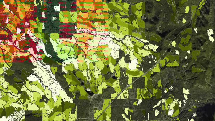
Visualization with the voxel layer is very effective and we can see changes in any horizontal slice or vertical slice; however, we don’t have an overview of all changes. Now let’s flatten the image cube by extracting the changes from the change analysis raster and creating a change map. There could be many types of changes in the forest, but we are particularly interested in pixels that are changed to water from 1984 to 2021. The extraction criteria can be described as decreasing change direction, with NDVI value change from a starting value in a range of 0.02 to 1 (vegetation) to an end value in a range of -1 to 0.01 (water), here very small changes are filtered out to reduce noise. We will use the Detect Change Using Change Analysis Raster tool with the defined criteria to create the change raster as seen below.

The change raster is rendered using a red to yellow color ramp and overlays on top of an image of the year 2021. This change map tells us not only the locations but also the years when changes occurred. The pixel values represent dates where red means the land cover was submerged in water in earlier years, and yellow means the land cover was submerged in water in recent years. You can see how the Amazon River has reshaped the landscape, where islands in the middle of the river shrunk or were lost, and forests along the river were submerged gradually and changed the river boundaries over the years.
")
Furthermore, we can quantify the change by calculating the change areas per year. The chart below shows the acreage of land cover submerged in water from 1985 to 2021, with the biggest change in 2009 and 2021 when large floods may have occurred. The total area that has changed to water totaled 187,253.2 acres.

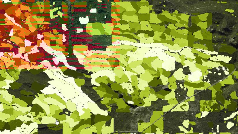
Using the same Detect Change tool with an increasing change direction, we can detect areas that changed from water to forest (or any nonwater land). The resultant change map (left picture below) is displayed on top of a 2020 image where the purple to pink image shows the time when forest or land “grew” from water. The middle picture is the input image of 2020, and the right picture is the input image of 1985. You can see the difference between the 2020 and 1985 images visually, but the change map we created quantifies the change, models the change progress, and provides more insight into the change in this area.

Discussion
This blog just analyzes a small area of the Amazon floodplain changes. Many more analyses can be done such as analyzing the different types of land covers involved in the whole change process and whether these changes are natural or anthropogenic. Since there are missing scenes for certain years due to cloud cover, leveraging other sensors or interpolating the data to fill those gaps may improve the analysis results. We hope this blog has provided you with the workflow and tools for image time series change detection and inspired you to further study this area or analyze land-cover change in any location on the planet.

Article Discussion: