Alaska occupies a unique place in the American imagination. It’s the largest state in the country, as well as the furthest north. It’s one of only two states unconnected to the mainland United States. Despite—or perhaps because of—these idiosyncrasies, the nature of Alaska’s size and location remain cartographically mysterious to many people. You see it perching sheepishly on maps, pinned haphazardly somewhere southwest of California, often miniscule in comparison to a state like Texas (which it is three times the size of).
Alaska as an idea is interesting, and its physical reality on the globe is also fascinating as a case study in mapmaking dilemmas. What can Alaska tell us about the shape of the planet and how it’s drawn on maps? Or, more germane to the Business Analyst Web App release of February 2024: What can Alaska tell us about hexagons as mapping tools?
In this article, we’ll zoom in (and zoom out) on Alaska, using it to examine the ways Business Analyst hexagons both deepen and, at times, limit its visual representation. We’ll look at size distortion, the problems presented by sparsely populated regions, and hexagons that sit on national borders. In the end, we hope you’ll approach hexagons with fuller knowledge and realistic expectations for what they can accomplish in your analyses.
All hexagons are [not] created equal
Hexagons provide a consistently sized grid across an area that does not change over time. Administrative boundaries in standard geographies do not provide this consistency as sizes can vary across an area and be redrawn over time. However, it can visually appear that a map using hexagons is distorted. For instance, using resolution 2 hexagons in Alaska paints a picture of larger hexagons in the north of the state and smaller hexagons in the south.

We can verify that the hexagons are consistent in size using the Measure tool. The Measure tool lets you measure the distance between points on the map and the polygon area.
First, let’s measure the distance between points in a hexagon in the northernmost compared to a hexagon in the southernmost hexagons in Alaska. I picked the northernmost hexagon and plotted a point on the West Coast and another on the East Coast. It measured 208.54 miles across in distance.

Then I picked a hexagon in a southern part of the state and repeated the process. The southern hexagon measured 209.73 miles across. This confirms that even though it visually appears that the hexagons in the northern part of the state are larger than the ones in the south, they are measurably consistent in size.

Another way to assess the hexagon size is by comparing the polygon area of two hexagons. I used the northernmost hexagon in Alaska again and measured its area using the Measure tool. It measured 35,918.26 miles squared, with a perimeter of 711.09 miles.

Then I picked the southernmost hexagon in the state of Texas and repeated the area measurement process. This hexagon measured 38,611.73 miles squared, with a perimeter of 740.58 miles. Visual distortion due to map projection is significant, but the areas are also approximately 10% larger. You should take care when using any calculations that use the hexagon area in custom variables.

Sparse data presents problems
Hexagons are an exciting mapping option for a lot of reasons, one being that they allow us to see the distribution of data independent of standard administrative boundaries that can distort our understanding of that data. But are there times when using standard geographic boundaries is preferable to hexagon mapping? Well…yeah. And here, again, Alaska can help us understand why.
Maps are only as informative as the data behind them. When an area is sparsely populated, apportioning data becomes more difficult, especially when not using the administrative geographies along whose lines the data was originally collected.
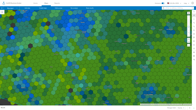
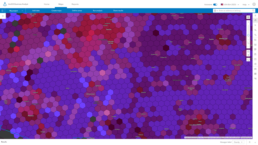
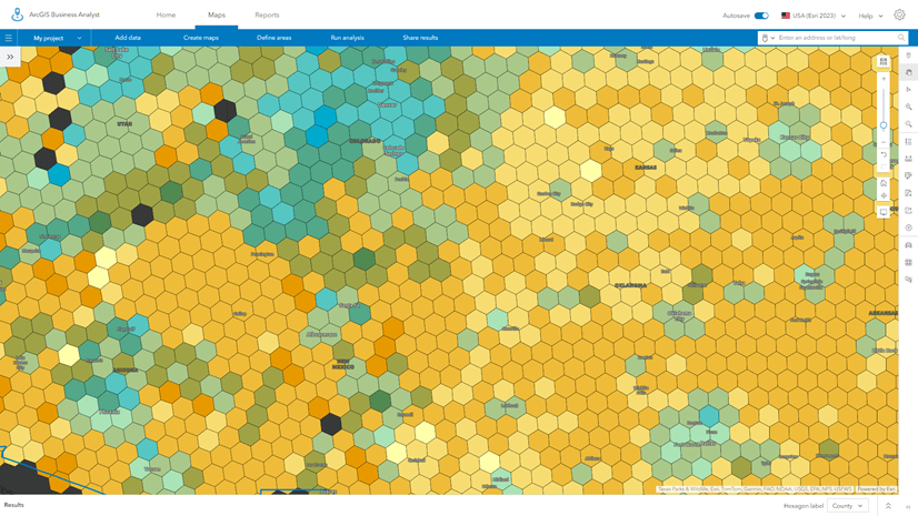
For example, I’ve mapped the variable 2021 Pop 3+ Enrolled Grade 9-12, an American Community Survey variable that captures the number and percentage of high schoolers in an area. I map the data at the county level first, then decide to see what it looks like in resolution 2 hexagons.

Initially, I’m thrilled to see more complexity in the data variation when I use hexagons—there are patterns here that I hadn’t noticed when using the county data. However, as I explore the hexagons, I notice some worrying things. For example, when I hover over a hexagon in the center of the state, I see there are 65 high school students living there—plus or minus 93 students.

Wait, what? As Diana Lavery and Lisa Berry point out in The Importance of Margins of Error and Mapping, such a large margin of error indicates less reliable data. The coefficient of variation is huge! When I switch to resolution 4 hexagons, I get a clearer picture of the problem.

There simply aren’t enough people living in parts of Alaska for the data to be reliably collected and apportioned. Where there is no data, there is no hexagon. This is not a problem unique to hexagons—standard geographies present similar hiccups for apportionment—but large hexagons can sometimes mask the problems hidden in smaller hexagons.
Hexagons across borders
As of February 2024, hexagons are available as a Business Analyst Web App mapping option in the United States. This means that, at times, hexagons appear to “bleed into” other countries where hexagons are not mapped. For example, Alaska borders on Canada in several spots:

While it may look a bit like each hexagon is summarizing the data in the entirety of the area covered, it’s important to note that the data values displayed are only for the United States. So, although, this resolution 2 hexagon covering part of Juneau indicates that the population living inside the hexagon’s bounds is 35,603—this is actually only the population inside the Alaska border (shown in blue).

It may seem like a footnote, and it will not be true forever (international border-spanning hexagons to come in a future release!), but understanding the data behind the hexagons can be helpful in your analysis. And if you’re interested in one more hexagon oddity, feel free to pan over the southwestern tail of Alaska at resolution 2, to get a peek at the International Date Line!
The IDL is a north-south longitude line exactly halfway across the world from the prime meridian. The International Date Line marks time as a calendar day; passing eastward decreases the date by one day.

Conclusion
In this article, we explored some unique ways in which hexagons are applied to Alaska. Hexagons in Business Analyst are an exciting new geography option with countless opportunities for enriched analysis.


Article Discussion: