Smart Mapping with Arcade: Exploring relationships

As of version 4.9 of the ArcGIS API for JavaScript (JS API), you can now generate relationship visualizations for FeatureLayer, CSVLayer, and SceneLayer. A relationship renderer, also known as a bivariate choropleth visualization, allows you to explore relationships that may exist between two numeric variables in a single layer. This post will cover the implementation details that allow the JS API to generate relationship renderers in web apps.

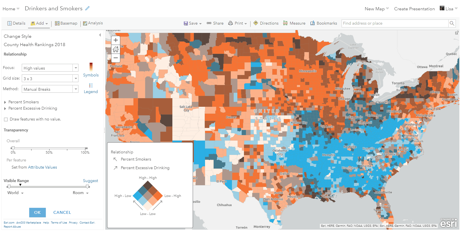
My colleague Lisa Berry wrote an excellent blog about relationship mapping in ArcGIS Online. I encourage you to read it before continuing this post. She describes the theory behind relationship maps and how to create one in ArcGIS Online in just a few clicks. Joshua Stevens also wrote this blog, which details the complexities, frustrations, and dangers involved with creating relationship maps, including working with class breaks, creating effective color ramps, and creating a legible legend.

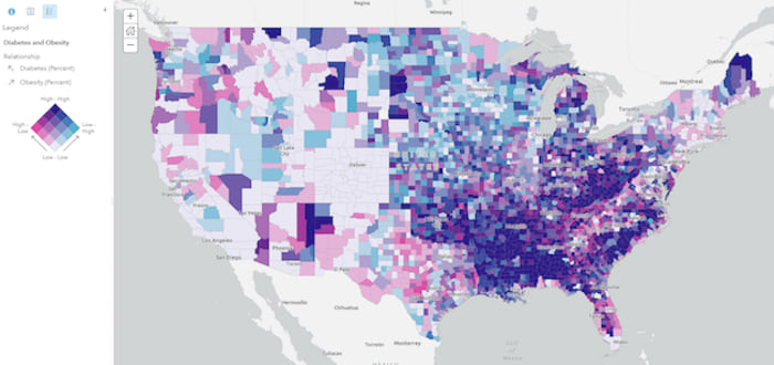
In Lisa’s blog, she explores the relationship between the U.S. population diagnosed with diabetes and the population classified as obese.

The typical legend that accompanies a relationship map is square-shaped. As with most visualizations, understanding the layout and colors of the legend is essential for communicating the message of any relationship map. Check out the image below which deconstructs a relationship legend to help us understand the reasoning behind its design.

Imagine you have two square legends for each numeric variable to visualize in the map (e.g. one for obesity, one for diabetes). Each variable has an associated single-hue color scheme with four class breaks representing quantiles of the data (classes with a range of 25% of the data). If one ramp is rotated 90 degrees then overlaid on the other, you get a square 4×4 grid of 16 categories.

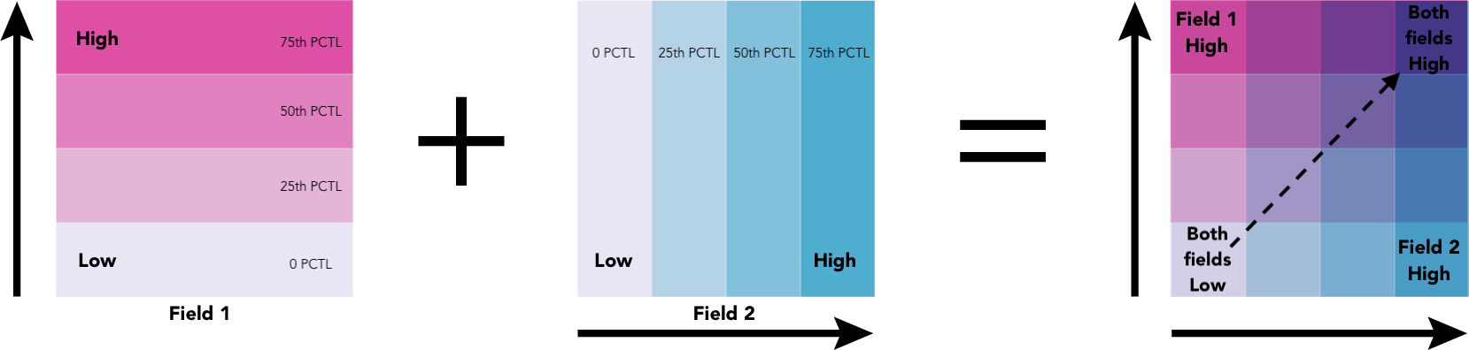
The overlay creates a third hue along a diagonal line from the bottom left corner to the top right corner. The colors along this line indicate features where the two attributes may be related or in agreement with one another. So features that have the deep purple color (labeled in the image with ‘both fields high’) indicate areas where the values of field 1 and the values of field 2 are higher than the 75th percentile of each respective field.

Bivariate color in 3D

This visualization style becomes particularly interesting in 3D because it’s often the only method for creating bivariate visualizations in 3D scenes. In traditional 2D visualizations you can achieve bivariate visualizations using a combination of color and size. In 3D, you can certainly use extrusions for thematic visualizations, but this isn’t possible for many layers because they contain 3D objects with mesh geometries, which already reserve the size visual variable for real world measurements. An example of this would be a SceneLayer of buildings where size can’t be altered because it would take away from the realistic nature of the buildings.

Even point FeatureLayers rendered with 3D WebStyleSybmols based on real-world sizes can take advantage of this technique to explore potential relationships between two variables.

Therefore relationship renderers can become particularly important for data exploration apps in 3D when size is already reserved for preserving the realistic scale of the feature.

Generate a relationship renderer for a SceneLayer

Relationship renderers are generated using the createRenderer method on the relationship Smart Mapping module. This method requires a layer, a view instance, and two fields.

const params = {
  layer: layer,
  view: view,
  basemap: map.basemap,
  field1: {
    field: "StarScore"
  },
  field2: {
    field: "ElectricUse"
  }
};

const response = await relationshipRendererCreator.createRenderer(params);
layer.renderer = response.renderer;

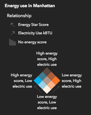
By default, the renderer is generated with three class breaks, forming a 3×3 grid in the legend. You have the option to change this to 2 or 4 class breaks. You can also specify a focus, which orients the legend as a diamond with the focus being the corner of the legend rendered at the top. This does not change the visualization on the map.

const params = {
  layer: layer,
  view: view,
  basemap: map.basemap,
  field1: {
    field: "StarScore"
  },
  field2: {
    field: "ElectricUse"
  },
  // HIGH field 1 value & HIGH field 2 value
  // corner of legend is on top
  focus: "HH",
  numClasses: 2
};

const response = await relationshipRendererCreator.createRenderer(params);
layer.renderer = response.renderer;

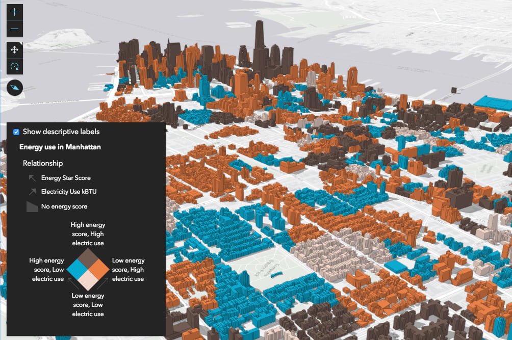
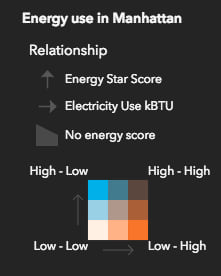
The code snippet above generates a renderer visualizing the relationship between the ElectricUse and StarScore (energy efficiency score) fields in a SceneLayer of New York buildings.

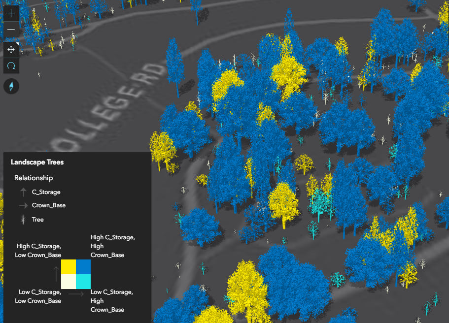
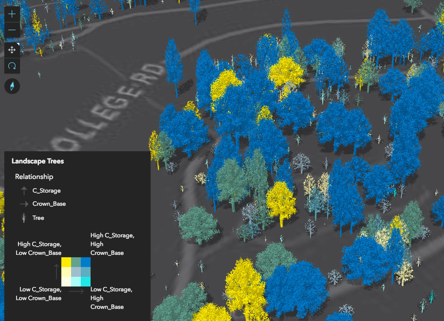
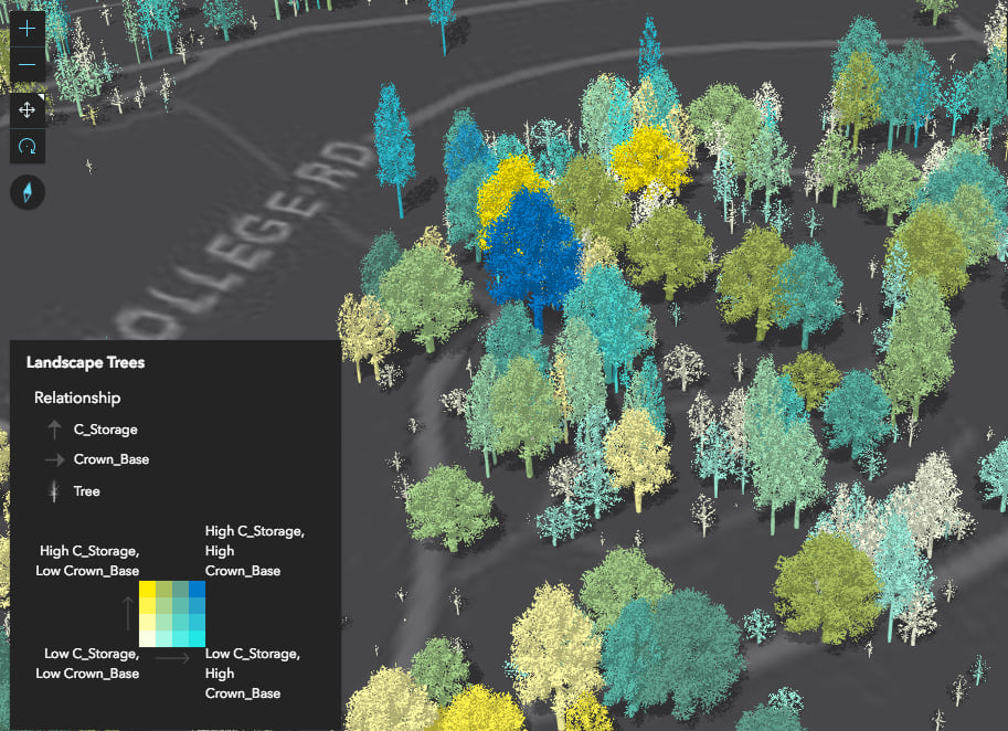
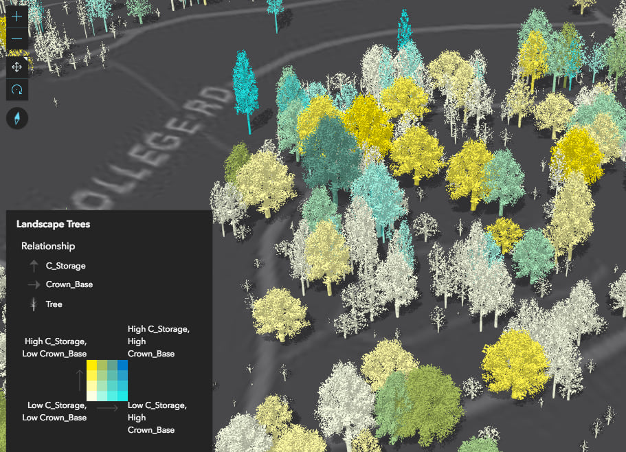
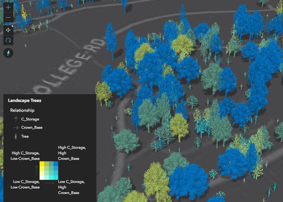
You can also create more involved data exploration applications, in which you allow the user to select one or more attributes to view their relationship with one another. The following app allows you to explore the relationship between a number of different variables in a dataset of trees.

The JS API provides other methods allowing you to create more complex data exploration applications. You can use these methods to give users control of the class breaks, color scheme, and legend text. This is exactly the level of control offered by the ArcGIS Online map viewer when you author a relationship visualization there.

How it works

Relationship maps can be difficult to get right. So we sought a method to make this easier. Most GIS software require you to complete several steps and a lot of trial and error to achieve a standard bivariate choropleth visualization. As noted above, with the relationship renderer creator module, all you need is a layer, two field names, and a view instance. That’s it! The API takes care of most of the guesswork for you.

So how do we do it? What’s going on behind the scenes? Rather than create a new RelationshipRenderer class, we decided to see if we could use APIs we already have as building blocks for this visualization.

If you inspect the output renderer from the response object of the tree data exploration app, you’ll notice that it isn’t a new renderer type at all. It’s actually a UniqueValueRenderer instance. The unique values are created based on generic names indicating which break a value belongs to for each field.

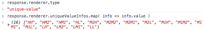
For example, LL stands for low-low. Features are classified this way if the value of each field falls into the lowest break for the respective field. HH represents the opposite scenario (high-high) where each field’s value falls into the corresponding highest class break. See the image below, which shows the placement of each of these generated values relative to the legend.

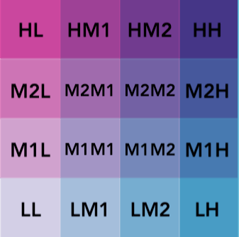
To generate these codes we first need to create class breaks for each field. This is done with the classBreaks method publicly available in the JS API. By default, the breaks are created using the quantile classification method. The main reason for this is because it makes the legend easier to read and describe. In a 4×4 legend, the top right corner represents features whose values for field1 and field2 both fall in the top 25% of their data distributions. If looking at the same corner of a 2×2 relationship visualization, then you can say both values fall in the top half of their respective distributions.

If you log the response object from createRenderer, you can view the class breaks generated for each field.

Quantile classifications don’t always work well. For that reason, you still have control over which classification method to use.

Once the class breaks are generated, the createRenderer method then generates an Arcade expression referencing the field names provided in the method parameters and assigns the proper code to each feature after matching the values of field1 and field2 to specific class breaks.

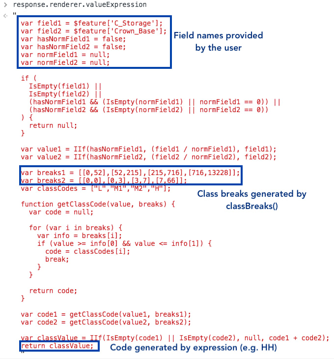
Once the Arcade expression and unique values are generated, the layer can render the bivariate color visualization.

Creating a legend

You don’t have to do anything extra to render the legend properly. Just reference the view in which the layer is rendered and the legend will display the relationship scheme as a grid.

const legend = new legend({
  view: view
});
view.ui.add(legend, "bottom-left");

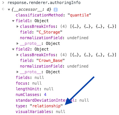
The Legend widget knows this is a special case and not a standard unique value visualization because the authoringInfo of the renderer indicates it is a relationship renderer.

By default, the legend displays generic text indicating where field1 and field2 have high and low values.

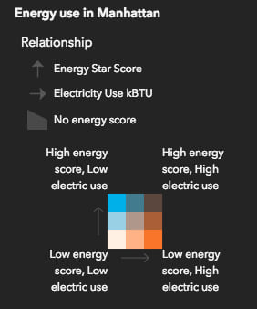
Since this default text isn’t useful to most users, you can modify it by altering the labels of the UniqueValueInfo objects for each corner value (e.g. LL, LH, HL, HH). Providing more useful text will better communicate the message of the visualization.

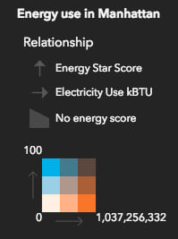
You could even display the min and max numbers for each range of values.

As mentioned above, you may also specify a focus to change the orientation of the legend so a particular corner is pointing upward. Or you could change the focus in the authoringInfo of the renderer to reorient the legend as you like.

The following function comes directly from the New York buildings app and executes each time the user checks or unchecks the checkbox just above the legend. When checked, the legend displays in diamond form with descriptive text. When unchecked, it re-renders as a square and displays numbers as if it were a chart.

function changeRendererLabels(renderer: UniqueValueRenderer, showDescriptiveLabels: boolean): UniqueValueRenderer {

  const numClasses = renderer.authoringInfo.numClasses;
  const field1max = renderer.authoringInfo.field1.classBreakInfos[ numClasses-1 ].maxValue;
  const field2max = renderer.authoringInfo.field2.classBreakInfos[ numClasses-1 ].maxValue;

  renderer.uniqueValueInfos.forEach(function(info: esri.UniqueValueInfo){
    switch (info.value) {
      case "HH":
        info.label = showDescriptiveLabels ? "High energy score, High electric use" : "";
        break;
      case "HL":
        info.label = showDescriptiveLabels ? "High energy score, Low electric use" : field1max.toLocaleString();
        break;
      case "LH":
        info.label = showDescriptiveLabels ? "Low energy score, High electric use" : field2max.toLocaleString();
        break;
      case "LL":
        info.label = showDescriptiveLabels ? "Low energy score, Low electric use" : "0";
        break;
    }
  });

  // When a focus is specified, the legend renders as a diamond with the
  // indicated focus value on the top. If no value is specified, then
  // the legend renders as a square

  renderer.authoringInfo.focus = showDescriptiveLabels ? "HH" : null;
  return renderer;
}

Relationship visualizations with thematic size

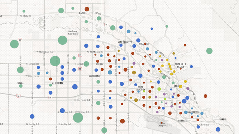
You can take 3D relationship visualizations a step further by adding a third variable to the mix if you’re working with data that doesn’t have an associated real world size. For example, take a look at the following app, which visualizes transit stops in Los Angeles with a relationship renderer. One variable indicates the percent of the population that belongs to a minority race, and the other is wait time for public transit during rush hour. The height of each point represents the total minority population living near the transit stop.

While more abstract, the added variable for height provides context to how many people in minority populations actually live in a given area compared to other transit stops.

Summary

The relationship renderer allows you to explore the relationship between two numeric attributes in your layer using only color as a visual variable. It is particularly useful for bivariate visualizations of 3D objects that can’t take advantage of other visual variables for bivariate purposes, such as size, which is already reserved for displaying features as they are in the real world.

Keep in mind that relationship visualizations have the same caveats as other single-variate choropleth maps, such as bias due to the number of class breaks, the classification method, and whether or not variables are properly normalized.

• 

• 

• 

• 

• 

• 

Be sure to use your best judgement when creating these visualizations. While the createRenderer method gives you a good starting point, you should still take time to update the legend text and make conscious decisions regarding the legend orientation, the number of classes, and classification method used to generate the breaks. Sometimes you will need to update the breaks manually. You can do this by updating the output Arcade expression.

If you have feedback for additional themes you’d like to see or try, drop us a note and we can try it out!